| Example | SIGNAL-SF (pub.) | SIGNAL-SF (ours) | # fam (pub.) | # fam (ours) | # EPT (pub.) | # EPT (ours) | %EPT (pub.) | %EPT (ours) |
|---|---|---|---|---|---|---|---|---|
| Lapstone Creek, Glenbrook 2024 | 5.00 | 5.00 | 15 | 15 | 1 | 1 | 0.50 | 0.49 |
| Hat Hill Creek, Blackheath 2024 | 7.14 | 7.14 | 17 | 17 | 6 | 6 | 77.10 | 77.11 |
| W. Falls Lake 2024 | 4.22 | 4.22 | 12 | 12 | 1 | 1 | 3.30 | 3.26 |
1 The monitoring record
Blue Mountains City Council Healthy Waterways — statistical analysis
1.1 What this chapter is for
Two databases, 27 years, 2,062 macroinvertebrate samples and 2,688 water quality samples. This chapter covers what is in them, how they join, what had to be repaired before anything could be analysed, and what they cannot be asked to answer.
It opens with the reproduction test, because everything else rests on it. We recomputed the four macroinvertebrate factors and the overall health rating from the raw taxon records, without going near the Access queries, and compared the result with what you publish. It matches — on every sample where a comparison is possible, and on all three worked examples in the June 2025 methods document, to the decimal. That is the licence for the other eighteen chapters. When a later chapter disagrees with a published figure, the disagreement is about the data or about the method; it is never about whether we implemented your system correctly.
Two other things to keep in mind before you read any result.
The monitoring network changed shape over 27 years. Different sites were visited in different years, so a plain year-on-year average of “waterway health” is partly a measure of which creeks were visited rather than of how the creeks are doing. Section 1.5 shows this directly, and it is the reason almost every model in the book carries a site term.
The family count double-counts some families. We found this by reproducing it rather than by disagreeing with it: the Access query relabels the chironomid subfamilies after de-duplicating, so a sample holding Chironominae and Orthocladiinae counts Chironomidae twice (Section 1.2). Your own Lapstone Creek worked example does it. It is reproduced exactly here, because the published bands were calibrated on the inflated count and changing one without the other would be worse than leaving both.
The object-by-object reference — what every table and function in the data layer is, the validation tables, and the house rules a future analysis has to respect — is Appendix A. This chapter is the description; the appendix is the manual.
1.2 Your published numbers reproduce, exactly
The waterbug database contains a chain of Access queries (CalcsStep1 … CalcsStep4, all marked DONOTEDIT) that derives the family counts, abundances and EPT figures you publish. Nothing in this report reads the output of those queries. We recomputed all of it from the raw Waterbugdata records and then compared, which is a much stronger test than reading the answers would have been.
1.2.1 The three worked examples
The June 2025 methods document works three samples end to end — every factor score, the average, and the resulting rating. They are the only complete specification of the system that exists outside the Access queries, so they are the test that matters most.
| Example | Average factor score (published) | Average factor score (ours) | Rating (published) | Rating (ours) |
|---|---|---|---|---|
| Lapstone Creek, Glenbrook 2024 | 1.50 | 1.50 | Poor | Poor |
| Hat Hill Creek, Blackheath 2024 | 4.00 | 4.00 | Excellent | Excellent |
| W. Falls Lake 2024 | 2.25 | 2.25 | Fair | Fair |
All three reproduce: the same eight factor scores (four, for the wetland), the same average, the same rating. Lapstone Creek averages 1.50 and comes out Poor; Hat Hill Creek averages 4.00 and comes out Excellent; Wentworth Falls Lake averages 2.25 and comes out Fair. The only differences anywhere in Table 1.1 and Table 1.2 are in the printed %EPT, and there are three of them: the document shows 0.5, 77.1, and 3.3 where the arithmetic gives 0.4902, 77.1084, and 3.2609. The document publishes %EPT to one decimal place where Table 1.1 prints two, so all three are presentation rounding in the document, and none of them moves a factor score.
These three are pinned in the data layer’s own tests by sample code — 2003, 2038, 2052 — and not by site and year, which is not a key here (Section A.1.2).
1.2.2 And on the whole series, not only on three samples
CalcsStep3A_C_OverallTotalsDONOTEDIT and CalcsStep4_EPT_DONOTEDIT). The strict family count is the one row expected to disagree: it is a different definition, not a failed reproduction.
| Quantity | Source | Compared | Agree | Agreement |
|---|---|---|---|---|
| Family count | Step 3A_C | 2,050 | 2,050 | 100.00% |
| Family count (strict, true families only) | Step 3A_C | 2,050 | 55 | 2.68% |
| Total abundance | Step 3A_C | 2,050 | 2,050 | 100.00% |
| Total abundance | Step 4 (TotalBugs) | 2,050 | 2,050 | 100.00% |
| EPT individuals | Step 4 (TotalEPT) | 1,956 | 1,956 | 100.00% |
| %EPT | Step 4 (%EPT) | 0 | – | – |
Family count, total abundance and EPT individuals agree on every sample where a comparison is possible — 100.00%, not 99-point-something (Table 1.3). The one row that does not agree is the strict family count, which is supposed to disagree; it is a different definition and it is described below.
One quantity could not be checked this way. The %EPT column of CalcsStep4_EPT_DONOTEDIT is empty in the SQLite conversion: not one of the 2,050 samples that have a Step 4 row carries a value in it — it was a calculated column in Access and did not survive the export — so %EPT is reconciled against the worked examples only. (That is 2,050 and not the 2,062 samples in the record because the twelve empty samples have no row in the Access chain at all — the same reason CalcsStep3A_1 returns 2,050, two sections below.) A re-export with that column filled in would close the last gap (dq:ept-percent-column-export).
1.2.3 How the family count actually works
Reproducing the family count meant reverse-engineering the query. CalcsStep1 is a SELECT DISTINCT over (site, date, sample, family, count) in which the five chironomid subfamilies are relabelled “Chironomidae” after the de-duplication, and in which Collembola, Ostracoda, Copepoda and Cladocera are excluded. The family count is then the number of surviving rows. Implementing that rule exactly matches your figure for all 2,050 samples that have one.
Three things fall out of it. None is a mistake we are correcting — they are described because they are the reason two different family counts exist in this book, and because the third one is genuinely odd.
Chironomids count more than once. A sample recording Chironominae = 46 and Orthocladiinae = 10 produces two rows both labelled “Chironomidae”, so Chironomidae counts as two families. This is what happens in the Lapstone Creek worked example, whose published count of 15 families includes Chironomidae twice.
Duplicate records are handled inconsistently. Where the same taxon is entered twice for a sample with different counts, both rows survive the
DISTINCTand the taxon counts twice; where the two counts happen to be identical, they collapse to one. Whether a taxon counts once or twice therefore turns on a coincidence in the abundance figures.The numerator and the denominator use different taxon sets. The family count excludes the four microfauna taxa; the total abundance and the %EPT denominator include them.
The size of it: across 2,050 non-empty samples the published family count exceeds a strict count of true family-level taxa by a median of 3 taxa (mean 3.01, range 0 to 14). Both are carried. n_families reproduces the published figure and drives the health rating; n_families_strict is the defensible ecological count. Chapters 13 to 16 come back to whether the strict count should replace it — the catch being that the published percentile bands were calibrated on the inflated definition, so swapping one without re-deriving the other would make things worse rather than better. Which of the three quirks you would actually want fixed is a question for you, not for us (dq:family-count-defects).
1.2.4 The rating, as implemented
health_score implements the rating exactly as the methods document sets it out. A stream sample gets eight factor scores — four against other Blue Mountains urban streams and four against reference streams — and a wetland sample gets four against a combined regional wetland comparison. The average of those scores maps to an ordered rating from Very Poor to Excellent.
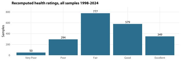
2,049 of the 2,062 samples are gradeable, and their mean average-factor-score is 2.872 — inside the Fair band, which is the middle class of a scale running 0 to 5 in five classes each 1.00 score points wide. The distribution is the one every later chapter works from, so here it is once: Very Poor 50, Poor 294, Fair 777, Good 579, Excellent 349.
The band tables are held as data rather than as code, so a different set of bands can be dropped into the same scoring (Section A.1). That is not a housekeeping detail. It is what makes chapters 14 and 15 possible: the revised bands proposed there are run through exactly the same scoring code as the published ones, so any difference in the answer is a difference in the bands and not in the arithmetic.
1.2.5 The samples that are no longer rated
Twelve samples have no taxon records at all. These are genuinely empty rather than missing — a visit happened and nothing was recorded — and they are absent from your own CalcsStep3A_1 family-count query too, which is why that query returns 2,050 rows and not 2,062. They are kept in every table with is_empty_sample = TRUE, zero counts and a missing SIGNAL average, because the mean grade of no families is undefined, not zero.
One further sample (750, Glenbrook Lagoon 2018) is not empty but recorded a single taxon, too few animals to score all four wetland factors.
All thirteen samples — the twelve empty ones and the partial one — used to receive a rating anyway. With four of the eight stream factor scores — or three of the four wetland scores — set to zero, they averaged 0.00 and were rated Very Poor. That is a zero meaning “nothing was found”, not “the sensitive animals were absent”, and those are different statements about a creek. They are now left unrated.
That single change is the whole of the difference between a Very Poor count of 63 — what the rating system produces if you let it score a partial factor set, and therefore the figure in anything computed before this report — and the 50 quoted here. Nothing has been deleted; the unmasked values are kept, and the rule for reconciling a figure against the old convention is in Appendix A.
Nine of the thirteen are consecutive sample codes (1579 to 1587), all from 2018, at nine different creeks. That is either a remarkable season or a lost laboratory batch, and nothing in the database says which — chapter 15 asks whether the field sheets survive (dq:unrateable-field-sheets).
1.3 The data behind this chapter
Each question and request below is set out again in What we need from you, with what it blocks, what an answer is worth and what it would cost you to find, ranked against every other ask in the report.
1.3.1 What this chapter uses, and where it came from
The rating system is implemented from the June 2025 methods document, including its three worked examples, which are the only end-to-end test of the implementation we have.
The document supplies the factor score tables, the desirable ranges, and the three-tier reference / slightly disturbed / urban site classification in its Appendix 2. None of those three attributes is in either database, so they are read from the document and carried on sites.
Blocks: Nothing. Value: low. Costs you: minutes. Refer to it as
dq:p-methods-document.
Everything in this report comes out of two of your Access databases — BMCC_WaterbugDatabase and WQDatabase — converted to SQLite and read without modification.
The waterbug side gives 2,062 macroinvertebrate samples at 134 sites from 1998 to 2024, with 31,271 taxon records and the CalcsStep1–CalcsStep4 query chain that derives your published figures. The water quality side registers 137 sites, 135 of which carry at least one sample, and gives 2,688 samples with 3,608 measurement rows. Nothing is written back: the SQLite files are read-only inputs and the originals are untouched.
Blocks: Nothing. Value: low. Costs you: minutes. Refer to it as
dq:p-two-databases.
1.3.2 What is wrong with it
129 of the 137 register sites now have a position good enough to delineate a catchment from; the remaining 8 have candidate positions far enough apart to give materially different catchments and are withheld rather than averaged.
An averaged position is a place nobody sampled. The eight are 27GLNR, L4, L13, M23, P7, U13, U39 and U44, and resolving them is the highest-value site question on this list.
Blocks: Any catchment, climate or fire covariate at those eight sites, two of which are reference sites. Value: low. Costs you: minutes. Refer to it as
dq:pr-eight-positions-withheld.
The published family count exceeds a strict count of true families by a median of 3 taxa, because each of the five chironomid subfamilies is relabelled “Chironomidae” after the de-duplication step, so one family can count up to five times.
Reproduced exactly from CalcsStep1, so this is a description of your calculation rather than a disagreement with it. Both counts are carried: n_families reproduces the published figure and drives the rating, n_families_strict is the defensible count. They must never be mixed inside one analysis.
Blocks: Nothing immediately — but the published percentile bands were calibrated on the inflated count, so any move to the strict count means re-deriving them. Value: low. Costs you: minutes. Refer to it as
dq:pr-family-count-inflated.
1.3.3 Questions only you can answer
A handful of sites carry a stored lat/lon and an easting/northing that point to different places — 81NFB by 580 m, and 35GFB, 18BKT, 80BMG and 41NWL by over 170 m. Which of each pair is right?
We would rather you adjudicated these than us: a wrong pour point is a wrong catchment, and the catchment is what everything else in the report hangs off. U39 is a separate case — its northing is six digits (626800) where it should be seven, and we have reconstructed it as 6262800. Tell us if that is wrong.
Refer to it as
dq:coordinate-pair-conflicts.
We found three quirks in the way the family count comes out of CalcsStep1. Which of them are deliberate, and which would you want fixed in the next version?
One, the five chironomid subfamilies are relabelled “Chironomidae” after the SELECT DISTINCT, so a sample with Chironominae and Orthocladiinae counts Chironomidae twice — your own Lapstone Creek worked example counts 15 families including Chironomidae twice. Two, where a taxon is entered twice for one sample with different counts both rows survive and it counts twice, but if the two counts happen to be identical they collapse to one. Three, the family count excludes Collembola, Ostracoda, Copepoda and Cladocera but the abundance and %EPT denominators include them. We have reproduced all three exactly and changed nothing; whether they should change is your call, not ours.
Refer to it as
dq:family-count-defects.
Eight sites have two or three plausible positions on the map. Which one is right? Start with 27GLNR — it is a reference site and its two candidates are 1.6 km apart.
The eight are 27GLNR, L4, L13, M23, P7, U13, U39 and U44 (SITE-SUBSETS.md is the register). For seven of the eight the rival positions are between 700 m and 2.1 km apart, which is far enough to give a materially different catchment, so we have withheld them rather than average them — an averaged position is a place nobody sampled. U39 is the eighth and a different problem: its register northing is 626800, six digits where a seven-digit MGA northing belongs. For most of these the register easting/northing picks one point and the creek name picks another, and that is not our call to make.
Refer to it as
dq:site-coords-ambiguous.
Are U42 and 07GBH (12 m apart), P2-M6 and 74EBB (24 m), and 32EWD and 32.2EWD (98 m) three sites recorded under two codes each, or six distinct sites?
As pour points each pair is one catchment, so the distinction matters for how the samples are treated: two codes on one site means the samples are not independent, and it also moves the published site counts. One of the three pairs, 32EWD and 32.2EWD, is also on the relocated-site pairs table in chapter 1 (Table 1.8), where the .2 code convention reads it as one site moved to a different reach rather than as one site coded twice. Those are two different answers to this question, and the relocation reading is the register’s convention rather than a confirmed fact, so answering this settles both.
Refer to it as
dq:duplicate-site-codes.
Fourteen pairs of site codes in the register are a relocation — 09BBH to 09.2BBH, 59BLA to 59.2BLA and twelve others. Do you want each pair reported as one continuous series, or as two?
A relocated site is a different reach, so we have kept them separate and flagged the relationship rather than splicing them. But you are the ones who will read the trend for Centennial Glen Creek, and if a break in the series at 2024 is going to confuse the reporting, that is worth knowing now. Either answer is fine; what we would rather avoid is the choice being made silently.
Refer to it as
dq:relocated-site-splice.
77EWD is recorded at 530 m, which puts it in the higher band by the methods document’s own under-500 m rule, but Appendix 2 assigns it to the lower band. Which one did you intend?
It changes that site’s conductivity and salinity desirable ranges and nothing else. We use the altitude-derived band and carry the Appendix 2 value alongside it so the choice can be tested either way.
Refer to it as
dq:site-77ewd-altitude-zone.
Can you confirm the town and creek behind the ambiguous codes? LN is used for both Lawson and Linden, C02 turns up in two coding schemes 2.9 km apart, and 32EWD is Garnett Dam but is typed as a stream in the register.
Anything joined on site code inherits these. The 32EWD one has a second consequence: a waterbody typed as a stream is scored against the stream trigger values and the edge band table, neither of which was derived for it. It also has two names in this report — Garnett Dam here, and Garnett Creek in the relocated-site pairs table (Table 1.8), which takes the name from the waterway column of the register. Whichever is right, one name would be better than two.
Refer to it as
dq:site-code-decoding.
Some samples carry the same taxon twice with two different counts. Is that two picks of the same sample, a correction that was never deleted, or a typing slip — and would the lab sheets tell us?
We sum them, which is the only choice that does not throw a record away, and the family count is left exactly as your query produces it. But the duplicates are the reason a taxon sometimes counts twice and sometimes once, so knowing what they are would settle the question above as well.
Refer to it as
dq:duplicate-taxon-rows.
Methods Appendix 2 lists a slightly disturbed site as 38.2NHV; both databases spell it 38.2NVH (Glenbrook Creek tributary, Valley Heights). Which is right?
We have assumed the document has the typo and mapped it to the database spelling, because 38.2NHV appears nowhere else. It matters because the slightly disturbed tier is half the population the desirable ranges were derived from.
Refer to it as
dq:appendix2-site-code-typo.
If a position genuinely cannot be recovered for a site, do you want to retire it formally — or leave it on the books?
Either answer is fine. What we would like to avoid is a site quietly dropping out of the analyses because nobody ever decided, and then somebody noticing in five years and asking what happened to it. It should be a decision you took, and the report should record it as one.
Refer to it as
dq:retire-orphan-sites-decision.
1.3.4 What would answer them
Were either of the Hazelbrook bifenthrin locations (87GHZ, 88GHZ) ever sampled before 2023, perhaps under an older site code? Even one visit would do.
There are two bifenthrin contaminations in this archive, eleven years and seventeen kilometres apart, and both are missing the same thing. The 2012 Jamison Creek kill has a control and two impact sites sampled together from five days after the kill was found out to 2024, which is the strongest thing here — but the control and the near impact site were both established after the event, so it has no “before” either (chapter 17). Hazelbrook is the same shape and smaller: the incident is recorded, the sampling only starts afterwards, so the pair is a description rather than a test. It is also the one where a pre-incident sample might plausibly still exist under an older site code, which is why the ask is here and not there. Fifteen minutes of somebody’s memory, or a look at the site register.
Refer to it as
dq:hazelbrook-pre2023.
Do the written site descriptions still exist for the ambiguous sites — the “Rian’s Pool, adjacent to the oval” ones? Who would have kept them?
A description like that is the only thing that lets a position be picked off imagery or a map. Without one, the choice between two candidate points cannot be made at all, by us or by anyone else. This is the enabling document for the question above rather than an ask in its own right.
Refer to it as
dq:site-written-descriptions.
Could someone re-export CalcsStep4_EPT from Access with the %EPT column populated? It was a calculated column and it came across empty in all 2,062 rows.
It is the one published quantity we cannot check against the whole series — we match your family counts, abundances and EPT counts on every sample, but %EPT only against the three worked examples. A five-minute export turns the last unchecked figure into a checked one.
Refer to it as
dq:ept-percent-column-export.
Is there a crosswalk between site codes and the geometry in the five bioindicators/ sampling-point layers and Firesites? None of them carry a site code.
These are layers you already hold and we already have copies of. Without a code on the geometry they cannot be joined to anything, so they are currently unusable — which is a shame, because they are the only spatial record of several sampling programs.
Refer to it as
dq:site-code-crosswalk.
Are there intact copies of AllMAcroSites22_8_18.TAB (its .DAT sibling is missing) and GISRRatings2018.TAB?
Low priority — we used the .xlsx twins instead and they were fine. It would give a fifth independent lineage to check the recovered coordinates against, which is the only reason it is on the list at all.
Refer to it as
dq:intact-site-tab-files.
Are the original field GPS records still anywhere? Stored precision runs from 1 m to 500 m — twelve sites are rounded to 100 m and two to 500 m.
A 500 m rounding cannot choose between candidate points 700 m apart, so several of the ambiguous sites are ambiguous only because precision was thrown away on the way into the database. Going forward the fix is simply to store what the handset gives you.
Refer to it as
dq:site-gps-precision.
1.4 The two databases and how they link
You keep two Microsoft Access databases, supplied here as SQLite conversions.
BMCC_WaterbugDatabase; ‘Water quality’ is WQDatabase.
| Database | Key tables | Contents |
|---|---|---|
| Waterbug | Sites, Samples, Waterbugdata | Macroinvertebrate sampling: 134 sites, 2,062 samples, 31,271 taxon records (1998–2024). |
| Waterbug | Signal, BMCCBugnames_SIGNAL, EPTList, TAXONOMY_FAMLEVEL | Taxon lookups: SIGNAL 2 and SIGNAL-SF sensitivity grades, EPT membership, family-level taxonomy. |
| Waterbug | CalcsStep1–4 (“DONOTEDIT”) | The Access queries that derive the published family counts, abundances and EPT figures. |
| Water quality | tblSites, tblSamples, tblWaterQuality | Water quality: 137 register sites (135 sampled), 2,688 samples, 3,608 measurement rows (1998–2025). |
| Water quality | tblSiteDescription | Habitat description at the time of sampling: shading, substrate, macrophytes, riparian structure. |
| Water quality | tblRecWaterQuality, tblProjects | Recreational water quality (enterococci) and project attribution. |
The two link on site code plus sampling date. Every one of the 134 macroinvertebrate site codes also exists in the water quality database; 3 further codes (921.1, 922, 926) appear only on the water quality side and are recreational-monitoring locations. That is the whole of the difference between the two, and it is the commonest way a site count goes wrong: 134 is the bug-monitoring network, 137 is the site register, and a count of one is not a count of the other. Nothing in this book counts sites by hand — Section A.1.3 is the reconciling table, and Section A.1 the rest of what the build produces.
1,840 of the 2,062 macroinvertebrate samples (89.2%) have a water quality sample taken at the same site on the same day. A further 36 have one within 30 days; those are not merged, but the nearest match and its lag in days are recorded, so an analysis can widen the window deliberately instead of by accident.
That headline is more generous than the working number, because a matched water quality record is not a matched water quality measurement. 124 of those matches point at a visit where nothing was in fact measured, so the usable rate is 1,716 (83.2%). For an analysis that needs all four core probe parameters at once it falls to 1,120, or 54.3% of the macroinvertebrate record. Every chapter that pairs bugs with water quality quotes its own per-parameter n for this reason.
A date-conversion trap that costs 268 matches.
Dates in both databases are stored as Unix epoch seconds written by a converter running on Sydney time. Macroinvertebrate sample dates land on exactly 13:00 or 14:00 UTC — midnight Sydney, in daylight saving and standard time respectively. Converting them with R’s default (
as.Date()on a date-time uses UTC) therefore moves every macroinvertebrate sample one day earlier. Water quality records from 2020 onward carry a real time of day and are unaffected, so from 2020 the two databases end up systematically one day apart. Under the default conversion only 1,572 samples match; with the Sydney time zone applied, 1,840 do. The data layer handles it. Anything reading the SQLite files directly has to do the same, and nothing in the data will tell you that you got it wrong — the answer is just quietly 14.6% smaller.
1.5 Temporal and spatial coverage
How much monitoring happened, and where, is not steady across the record.
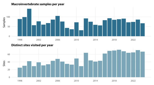
The two panels of Figure 1.2 do not move together. The sample count swings by a factor of 4.6 across the record, the site count by 2.9, so a year can be busy at few sites or thin across many. Both matter, and they matter differently.
1.5.1 The unbalanced panel
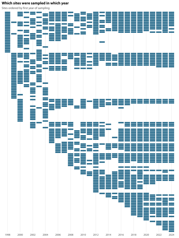
The single most important thing to know about this dataset is that the set of sites monitored changes from year to year. Statisticians call that an unbalanced panel, and it is not a defect in the monitoring — it is what 27 years of a real program looks like. It does mean that some obvious ways of summarising the data give the wrong answer. Figure 1.3 shows every site against every year; each filled cell is a year in which that site was sampled at least once.
| Panel start | Years | Sites sampled in every year |
|---|---|---|
| 2006 | 19 | 0 |
| 2010 | 15 | 1 |
| 2012 | 13 | 16 |
| 2015 | 10 | 30 |
| 2017 | 8 | 51 |
No site was sampled in every year from 2006 to 2024. Insisting on a balanced panel therefore costs either sites or years (Table 1.5): you are left with 16 sites if you start in 2012, 30 if you start in 2015 and 51 if you start in 2017 — against 134 sites in the network.
Why this matters in practice: if the average health score rises from one year to the next, that can happen because the creeks improved, or because a different set of creeks was visited. The two are indistinguishable in a raw annual mean, and the composition effect here is large — the network more than doubles in size across the record.
What a site random effect does, since most of this book uses one. Instead of averaging every sample together and hoping the site mix cancels out, the model gives each site its own baseline level and then asks what is left over after those baselines are taken out. The year-to-year change is estimated within sites, from creeks compared against themselves, so a year that happens to include more good creeks does not read as an improvement. The cost is that it assumes the site baselines are drawn from a common distribution, which is a mild assumption here and a very useful one: it lets a site with two samples contribute what it can without pretending to be as informative as a site with twenty. Where a chapter uses a balanced panel instead, it says so, and it says which one.
The house rule that follows from it is collected with the others in Appendix A, and every chapter in this report says which panel or which site term it used.
1.5.2 Which sites, and where they are
| Category | Sites |
|---|---|
| Sites in the macroinvertebrate database | 134 |
| Core reporting sites | 27 |
| Currently active sites | 75 |
| Historic (register note reads ‘Historic’) | 31 |
| Reference sites | 17 |
| ‘Slightly disturbed’ sites (methods Appendix 2) | 22 |
| Wetland sites | 9 |
Two of the categories in Table 1.6 are not in either database. The three-tier reference / slightly disturbed / urban classification the desirable ranges were derived from, and the altitude band that selects the conductivity and salinity ranges, both come from Appendix 2 of the methods document; the databases carry only a coarser four-way Classification field and a recorded altitude. The historic flag is ours, read off the site register’s notes field where it reads exactly Historic — it is not a rule about the site code. The 31 sites it selects span six code prefixes, of which the legacy K, L and M series account for seventeen. Core reporting sites and currently active sites are Council’s own designations, carried through unchanged.
Two places where the document and the databases disagree. Appendix 2 lists a slightly disturbed site as 38.2NHV; both databases use 38.2NVH (Glenbrook Creek tributary, Valley Heights), which appears to be a typo in the document and is mapped as one (dq:appendix2-site-code-typo).
And one site disagrees on altitude zone:
| Site | Waterway | Altitude (m ASL) | Zone from altitude | Zone in Appendix 2 |
|---|---|---|---|---|
| 77EWD | Wilsons Glen Creek | 530 | higher | lower |
77EWD (Table 1.7) is recorded at 530 m, which puts it in the higher band by the document’s own under-500 m rule, yet Appendix 2 assigns it to the lower band. We use the altitude-derived value and carry the Appendix 2 value alongside it (altitude_zone_appendix) so a chapter can test whether the choice matters. It moves one site’s conductivity and salinity ranges and nothing else (dq:site-77ewd-altitude-zone).
Where the sites are. The coordinates were never missing. easting and northing are populated for every one of the 137 register rows and every one of the 134 waterbug rows. What was sparse is the stored Latitude/Longitude pair — 85 of the 137 register sites, 82 of the 134 bug sites — and that pair used to be the only position the data layer read. That is the whole of why 52 sites have been called unlocatable. Reading the eastings and northings instead recovers 44 further positions.
So 129 of the 137 register sites — 126 of the 134 bug sites — now have a position good enough to delineate a catchment from. The remaining eight (27GLNR, L4, L13, M23, P7, U13, U39, U44) have candidate positions far enough apart to give materially different catchments, and are withheld rather than averaged, because an averaged position is a place nobody sampled. Resolving them is one of the two site questions this chapter rates high value, and the more expensive of the two to answer (dq:site-coords-ambiguous). A further seven sites carried two stored positions more than 100 m apart and were adjudicated one at a time against the DEM, the creek lines and the recorded distance from source; the eastings and northings won five of the seven (dq:coordinate-pair-conflicts).
None of the 44 newly positioned sites is a current monitoring site, and all of them are pre-GPS codes, so this is a recovery of the early record rather than a correction to anything being sampled now. Each of these counts, and the population it is taken out of, is in Section A.1.3.
Relocated sites. Your convention is that a code of the form NN.2XXX replaces NNXXX when a site has to move, for safety, access or habitat reasons. Fourteen pairs in the register follow it:
| Earlier site | Replacement site | Waterway | Location |
|---|---|---|---|
| 05GMVR | 05.2GMVR | Asgard Brook | D/S of Asgard Swamp trail crossing |
| 09BBH | 09.2BBH | Centennial Glen Creek | Upstream Centennial Falls, d/s trib junction |
| 15GKT | 15.2GKT | Yosemite Creek | Minnehaha Falls Reserve |
| 17GLA | 17.2GLA | Govetts Creek | Via Sewage Pumping Stn 75 Rawson Pde |
| 22BWF | 22.2BWF | Lillians Glen | Via West/Bate St |
| 23BWF | 23.2BWF | Jamison Creek | Weeping Rock |
| 25GWF | 25.2GWF | Wentworth Creek | Evans St firetrail (Bruce’s Walk track) |
| 28EHZR | 28.2EHZR | Ingar Creek | D/S Ingar campground |
| 32EWD | 32.2EWD | Garnett Creek | Not recorded |
| 37NSP | 37.2NSP | Magdala Creek | Fairy Dell Track |
| 38NVH | 38.2NVH | Glenbrook Creek tributary | Valley Heights |
| 43NYK | 43.2NYK | Frasers Creek | U/stream of Yellow Rock tributary junction, via Yellow Rock Creek Trail |
| 45NBX | 45.2NBX | Cripple Creek | 920m downstream of landfill |
| 59BLA | 59.2BLA | Leura Falls Trib u/s Chelmsford Dr | Leura Falls Creek Tributary |
A relocated site is a different reach of the creek, so the data layer flags the relationship and deliberately does not merge the two series (the house rule). Whether you would rather see them reported as one series is a decision worth making explicitly rather than by default (dq:relocated-site-splice).
One caveat on Table 1.8. 32EWD and 32.2EWD are read as a relocation here because they follow the code convention, but the same pair is 98 m apart and appears earlier in this chapter’s data section as a candidate for one site recorded under two codes (dq:duplicate-site-codes). Only one of those readings can be right, and the convention is not evidence.
1.6 Taxonomy reconciliation
Three separate things had to be reconciled before a taxon name could be counted: the spelling of the name itself, how coarsely the animal was identified, and whether the index used to score it has a grade for it at all. None of the three is a defect in the recording. All three change what a family count or a sensitivity score means, and the third changes it over time.
1.6.1 Taxon names
| Name as recorded | Records | Fixed by normalising? | Matches SIGNAL lookup? |
|---|---|---|---|
"oligochaeta" |
120 | yes | yes |
"ostracoda" |
78 | - | NO |
"Ostracoda" |
48 | - | NO |
"Copepoda" |
30 | - | NO |
"Cladocera" |
29 | - | NO |
"isopoda" |
25 | yes | yes |
"Spercheidae" |
2 | - | NO |
"Stratiomyidae " |
2 | yes | yes |
"Gomphomacromiidae" |
1 | - | NO |
Matching taxon names on a lower-case, whitespace-trimmed key resolves oligochaeta, isopoda and Stratiomyidae (trailing space) in Table 1.9. That leaves six name variants genuinely absent from the SIGNAL lookup:
ostracodaandOstracoda(two case variants of one taxon),CopepodaandCladocera— microcrustacea, recorded only sporadically. These are not family-level identifications, which is why the ordinations drop them: the AUSRIVAS manual identifies Ostracoda to subclass (Turak et al. 2004), and mixing a subclass with families confounds taxonomic resolution with composition. Copepoda and Cladocera carry no AUSRIVAS taxa code and no SIGNAL grade at all.Spercheidae(2 records) andGomphomacromiidae(1 record) — real families that were never added to the SIGNAL grade table.
Collembola is a separate case and is not one of those six: it is in the SIGNAL lookup but excluded by the calculation chain (Section 1.2).
All of these are kept rather than dropped, and flagged, so a chapter that wants them out takes them out deliberately. They carry no SIGNAL grade, which is the next section’s problem.
EPT membership is a second place where two definitions had to be reconciled: it comes from the EPTList table, cross-checked against order membership in TAXONOMY_FAMLEVEL, and the two agree on every taxon that occurs in the data.
1.6.2 Family-level versus coarse identifications
| Category | Taxa |
|---|---|
| Distinct taxa recorded | 138 |
| True family-level identifications | 119 |
| Coarse taxa (order or higher) | 14 |
| Chironomid subfamilies (finer than family) | 5 |
Not every record is identified to family (Table 1.10). Oligochaeta, Acarina, Amphipoda, Isopoda, Nematoda, Hirudinea, Turbellaria and the microcrustacea are order-level or higher. In the other direction the Chironomidae are often recorded as subfamilies, which is finer than family. Both matter for a metric called “number of families”, and both are why Section 1.2 has two of them.
1.6.3 SIGNAL-SF coverage over time
Two sensitivity indices run through this report and they are not the same thing. SIGNAL is the family-level biotic index in which each family carries a sensitivity grade and a sample’s score is the mean grade of the families present (Chessman 1995). The original grades were expert judgement; they were later re-derived from field data against measured water quality (Chessman et al. 1997) and then revised nationally as SIGNAL 2 (Chessman 2003), which is the version in general Australian use. SIGNAL-SF is the short-form variant your rating system uses, and it grades a smaller set of taxa. One of the two papers that introduced SIGNAL tested it on the Nepean and on Blue Mountains creeks (Growns et al. 1995), so the index was shown to work on the water you monitor early on. That is a demonstration of local relevance, not a calibration: the grades were not fitted here.
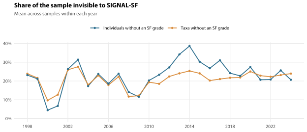
SIGNAL-SF grades are missing for 91 of the 233 names in the SIGNAL lookup, overwhelmingly the coarse taxa — Oligochaeta, Acarina, and Chironomidae when not identified to subfamily. Those taxa simply drop out of the average.
Across the 27 years the mean proportion of taxa in a sample carrying no grade runs from 10% to 28%, and the proportion of individuals from 4% to 39%, peaking in 2014. A change in how much of the sample the index can see is a change in the index, whatever the creek is doing, so this is a real confound for any SIGNAL-SF trend.
And the four years the index appears to see best — 2000, 2001, 2008, 2009 — are the four years chironomid identification practice changed. Chironomidae is the largest single ungraded group, so when it is recorded coarsely or not at all, prop_count_no_sf_grade drops for a reason that has nothing to do with grade coverage. In those years the column measures identification practice, and a model using it as a covariate is partly controlling for the wrong thing. Chapter 3 owns this: it sets out what happened in each of those years, how large the effect on the family count and %EPT is, and what a chironomid-free sensitivity check does to the answer. What every other chapter has to do about it is the chironomid caveat.
1.7 Water quality
The water quality side of the record is in materially worse condition than the macroinvertebrate side. It is still usable — most of it, for most purposes — but it needed more repair, and the repairs are set out here once so that every later chapter can work from the same description. Nothing has been deleted, substituted or imputed: where a reading has been set aside, the sample it belongs to carries a flag saying so, and the counts all appear in the validation table in Appendix A (Section A.1).
1.7.1 Repeated readings
| Probe readings per sample | Samples |
|---|---|
| 1 | 1,150 |
| 2 | 76 |
| 3 | 703 |
| 4 | 32 |
| 5 | 3 |
| 6 | 6 |
tblWaterQuality holds 3,608 rows for 1,981 distinct sample codes, not one row per sample. A further seven rows carry no sample code at all; every populated field in them is zero, so nothing is lost, but they can be joined to nothing. The extra rows are replicate probe readings taken minutes apart at the same visit — 703 sample codes have exactly three (Table 1.11), which is standard practice with a multiparameter probe. They differ mainly in the recorded time and the probe values; the laboratory parameters (alkalinity, phosphate, nitrate-N, faecal coliforms, ammonium) are usually entered once and left blank on the remaining replicates.
What we did: aggregate each sample to one row by taking the mean of each parameter over its non-missing replicates. For probe parameters that averages the replicates, which is what they are for. For laboratory parameters a single replicate is usually populated, so the mean of one value is that value — but not always. 326 (parameter, sample code) pairs carry more than one populated laboratory result (alkalinity 45, phosphate 67, nitrate-N 67, faecal coliforms 16, ammonium 131) and have been averaged, so for those the stored value appears in no laboratory record. Where the two results differ, anyone reading an individual site visit off a table has no way of telling that the number is an average. Every affected case is identifiable, and Section A.1.2 says which column to read to find them.
Faecal coliforms are averaged arithmetically even though plate counts are log-normal and the ANZECC/ARMCANZ guidelines express every coliform figure as a median (ANZECC and ARMCANZ 2000). (Geometric means for faecal indicators are the formulation of the recreational water guidelines, a separate document; ANZECC Volume 1 does not use them for coliforms.) That affects 16 sample codes; changing the rule is your call rather than ours, and chapter 7 puts the question (dq:coliform-mean-decision).
718 of the 2,688 water quality samples have no measurement row at all; 434 of those are recreational samples whose results live in tblRecWaterQuality. They are kept with has_measurements = FALSE rather than dropped, so a sample count is never silently a measurement count.
1.7.2 Six things that had to be repaired
1. A large block of laboratory results is left-censored — that is, the reading is not a measured concentration but a statement that the concentration was below what the method could see. No reading in tblWaterQuality is stored with a <; every parameter column is numeric, and a below-limit result is written as a plain zero. The < survives only in the field notes — a Lawson Creek sample of 12 September 2008 reads “Phos <0.1, Nitrate <0.1” and a Grose River tributary sample of 13 February 2009 reads “Phos<0.01, Nitrate <0.01”, and both are stored as 0.0. So there is a large block of readings at or below the limit of the method, written as exact zeros, which behave exactly like non-detects. The flags test each reading against its parameter’s detection limit where one is known, rather than looking for zeros, because for faecal coliforms the convention changed part way through the record.
| Parameter | Measured | Non-detects | Detection limit |
|---|---|---|---|
| Phosphate (ppm, as PO4 or as P) | 1,127 | 606 (53.8%) | 0.01 (inferred) |
| Faecal coliforms (CFU/100 mL) | 1,119 | 471 (42.1%) | 10 (confirmed) |
| Nitrate-N (ppm) | 1,029 | 56 (5.4%) | 0.01 (inferred) |
| Ammonium (mg/L) | 134 | 73 (54.5%) | none inferred |
| Alkalinity (ppm CaCO3) | 1,238 | 4 (0.3%) | none inferred |
⚠ Nothing records which phosphate the phosphate column is. The field is AvailPhosphate and the unit is ppm, and neither database, nor the field sheets, nor the methods document says whether that is phosphate expressed as PO4 or as P. The two differ by a factor of three, so every phosphate concentration in ppm anywhere in this report — the detection limit above, the desirable range in Table 1.13, and any level a later chapter quotes — means one thing under the first convention and a number three times smaller under the second. Counts, shares and rates of change taken from that same column are untouched by it, and so are pass rates against the 2024 desirable ranges, which were derived from percentiles of these same readings so that both sides of a pass or a fail carry whatever convention the kit used. Nitrate-N declares its species in its name and phosphate does not, which is the whole of the difference between them. Chapter 7 (Section 7.5) sizes the ambiguity where it bites hardest, and dq:phosphate-units is the one-line question that would settle it.
One of the five parameters in Table 1.12 has a confirmed limit. Faecal coliforms are censored at 10 CFU/100 mL, and the field notes in tblSamples say so directly — “FC <10CFU/100ml” against a recorded value, and, in July 2024, “0 colonies in 10ml but 1 in 1ml sample” against a recorded 100. A 1 mL and a 10 mL aliquot are plated and the colony count multiplied by 100 and by 10, so 10 is the smallest number the method can produce. That matters more than it sounds, because from 2020 a non-detect started being written down as 5 rather than 0, and a flag that only caught the zeros would have shown the non-detect rate halving from 2021 with nothing happening in the creeks. The coliform flag therefore catches everything below the limit, however it was written, and stands at 471 of 1,119 readings (42.1%).
The phosphate and nitrate limits are shakier. Neither is documented anywhere. Both are inferred at 0.01 ppm from the grid the results were written on: no phosphate or nitrate value below 0.01 ppm exists in tblWaterQuality in any year, the smallest positive reading of each is 0.01 ppm, and the readings step in units of 0.01 for twenty-two years without a break.
The ten values in the analysis data that sit under that grid — seven phosphate and three nitrate-N, all between 22 February and 27 April 2012 — are not readings. Each is exactly half a grid step, because each is the average of a laboratory duplicate in which one replicate read zero and the other 0.01.
What the grid establishes is the resolution the results were recorded at, not the floor of the method that produced them, and those need not be the same number. The only two surviving statements of a floor are field notes, and they disagree by a factor of ten: “Phos <0.1, Nitrate <0.1” in September 2008 and “Phos<0.01, Nitrate <0.01” five months later, each written beside a stored zero. So the limit is unconfirmed rather than unstable, which is the better of the two problems — but it is unconfirmed in both directions. 0.01 ppm is the finest thing the record can express; the true floor may be coarser than that, and nothing here can rule it out. Chapter 3 works out what the choice of floor does to the estimates.
That the phosphate zeros are non-detects at all — rather than measured absence — is supported from outside this database. A regional laboratory sampling the same catchments to the AUSRIVAS protocol recorded total phosphorus below its own stated limit in most of its Blue Mountains samples, with an explicit < where your database has a zero. It is an argument by analogy, across a different determinand and a period that does not overlap yours; chapter 7 (Section 7.5.1) sets out both the evidence and its limits.
Each of these five parameters is flagged where it is censored, and nothing is substituted or modelled away — that is a deliberate choice rather than an oversight, and the reasoning is in Appendix A. What no chapter here does is report “phosphate is within the desirable range in 76% of samples” — 1,044 stream comparisons across the whole record — without saying that just over half the readings are non-detects. As written, that is a statement about detection frequency dressed as a statement about concentration. Chapter 7 quotes a different and higher figure for the same parameter because it scores the 2022–2024 report-card window rather than the whole record; both are pass rates and neither is a concentration.
Confirming the remaining limits, and the date any test kit changed, is the single cheapest thing that would improve the water quality series: wq_detection_limits$confirmed is still FALSE for four of the five parameters, and the field notes that settled the coliform limit suggest the rest are findable (dq:lab-detection-limits).
2. Impossible values were screened out before aggregation. 641 raw readings failed a documented plausibility screen and were set to NA before the replicate averaging above, so that an impossible reading could not contaminate its sample’s mean: 568 total dissolved solids, 68 conductivity, three pH, one salinity and one turbidity. Nothing is destroyed silently — the bounds and the per-reading flags are both in the data layer (Section A.1). The bounds are deliberately generous: they exclude only the physically impossible, never the merely unusual, so a 185% dissolved oxygen saturation from a wetland bloom and a 41.9 °C summer reading both survive. This screen moves published figures: pH now runs from 3.53 rather than from 0.033 (a “pH” of 0.033 is a millivolt reading), the 2006 median conductivity is 45.5 µS/cm rather than 0, the salinity maximum is 0.59 PSU rather than 18.2 (which is half seawater), and the turbidity maximum is 658 NTU rather than 3,014.8.
3. Total dissolved solids change units by a factor of 1,000 in 2021. The Aqua TROLL writes g/L into a column named TDS(mg/L) from 1 January 2021. The TDS-to-conductivity ratio is about 0.645 for 2017 to 2020 — the textbook mg/L relationship — and 0.00065 from 2021. A harmonised series was built alongside the stored one (n = 1,004, median 47.5 mg/L); which of the two to analyse is a house rule, because the stored one looks perfectly usable and is not.
4. Pre-2020 salinity is quantised at 0.01 PSU. 776 samples are recorded on a 0.01 PSU grid against 954 at full precision. The published higher-altitude desirable range is 0.02 to 0.03 PSU — one quantisation step wide — so no exceedance rate or trend computed on pre-2020 PSU values is interpretable. The affected samples are flagged, and electrical conductivity, recorded to 0.1–1 µS/cm throughout, is the salinity indicator used across the whole series here.
5. Ammonia and total suspended solids are withheld. tblWaterQuality holds 423 non-missing nh3 values and 68 tss values, and every populated value is exactly 0.000. Both columns are withheld from wq so that no chapter can report “mean ammonia 0.000 mg/L across 148 samples” out of what is in effect an empty column. Neither database can support any statement about ammonia or total suspended solids. ammonium is a real, if sparse, series (134 samples) and is retained.
6. A handful of individual readings are data entry, not measurement. Every value in both databases was written on paper and then typed in, and nineteen individual readings did not survive the trip: a dissolved oxygen cell holding, to the digit, the turbidity value in the column beside it; a conductivity of 16 µS/cm between two replicates of 166 and 167 taken two minutes later; an alkalinity written as a literal 1 in a season where the other replicate of the same water reads 11.5 to 70. Each was identified by another reading of the same water contradicting it, never by being unusual on its own, and each is documented with its evidence in wq_transcription_suspect and in audit/TRANSCRIPTION-ERRORS.md. They are set to NA before the replicate averaging, because the averaging is what makes them dangerous: one mis-typed cell otherwise moves the stored value of a whole sample.
Those nineteen readings sit in eighteen (sample, parameter) pairs — one sample had two bad readings of the same parameter. In the fourteen pairs where a good replicate survived to say so, the bad cell had moved the sample’s stored value by between 40% and 139%. The other four had no surviving reading of that parameter, so those samples are now missing it rather than carrying a wrong value. The affected samples are flagged, and chapter 6 (Section 6.3.3) tabulates the before-and-after values.
Nineteen bad cells is a very low rate for 27 years of hand-entered records, and it reads as reassurance rather than as alarm. The rest — values that look suspect but that nothing in the data can correct — is left in place, flagged rather than altered.
Two more breaks are documented and not corrected, because correcting them needs information the databases do not hold: turbidity is dominated by which instrument was in the water rather than by the water, and faecal coliforms step by about a hundredfold across the summer of 2004–05. Both are chapter 3’s, which dates them, sizes them and says what a trend crossing either of them is worth; what every chapter has to do about it is the instrument-era rule.
1.7.3 Trigger values
| Parameter | Altitude zone | Desirable range | Measurements |
|---|---|---|---|
| pH | all | 5.28 to 6.75 | 855 |
| Turbidity (NTU) | all | 0 to 7.08 | 777 |
| DO (% saturation) | all | 77.2 to 100.09 | 827 |
| DO (mg/L) | all | 7.64 to 10.37 | 830 |
| EC (µS/cm) | lower | 71.05 to 178.6 | 262 |
| EC (µS/cm) | higher | 33.96 to 78.2 | 560 |
| Salinity (PSU) | lower | 0.03 to 0.07 | 262 |
| Salinity (PSU) | higher | 0.02 to 0.03 | 557 |
| Alkalinity (ppm CaCO3) | all | 4 to 16 | 368 |
| Phosphate (ppm, as PO4 or as P) | all | 0 to 0.044 | 369 |
| Nitrate-N (ppm) | all | 0.04 to 0.176 | 368 |
| Faecal coliforms (CFU/100mL) | all | 0 to 20 | 354 |
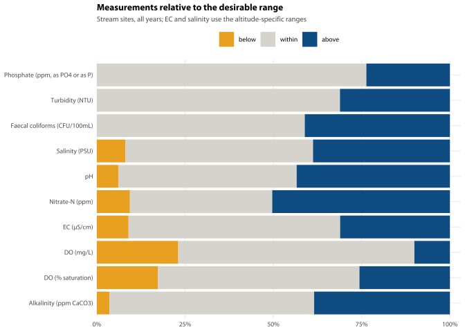
Electrical conductivity and salinity are compared against the altitude-zone-specific ranges of Table 1.13; 433 conductivity and salinity measurements come from sites with no recorded altitude and so have no applicable range at all. Figure 1.5 is the raw picture only; chapter 7 turns these comparisons into the report card, with the censoring and the instrument eras accounted for (Section 7.4).
These are early-warning triggers, not compliance standards. A result outside the desirable range is a condition worth following up, not a breach. The ranges follow the ANZECC and ARMCANZ framework, in which default trigger values are the 80th and/or 20th percentile of a regional reference distribution — the 80th for stressors that do harm at high concentrations, the 20th for those that do harm at low ones, and both together as a band only for stressors like pH, temperature and salinity that do harm at either end — and an exceedance is a prompt to investigate rather than a finding of harm (ANZECC and ARMCANZ 2000); the guidelines call the choice of cut-point “arbitrary (though reasonably conservative)” in the same passage. Deriving locally relevant values from local reference sites, which is what you have done, is what those guidelines recommend in preference to their own national defaults.
The published ranges are for streams. 2,500 of the 15,633 stored comparisons are wetland samples being judged against ranges derived from a site list of 32 stream sites and two wetlands — a stream distribution with a token of wetland in it rather than a wetland benchmark. They are kept and flagged rather than dropped, and they are excluded from the figure above. Chapter 11 takes up what that costs and what a wetland-specific set of ranges would need.
Provenance
| Item | Value |
|---|---|
| Data layer built | 2026-08-30 12:56 |
| R version | R version 4.4.3 (2025-02-28) |
| Source databases | BMCC_WaterbugDatabase_converted.sqlite (2025-08-05 11:26); WQDatabase_converted.sqlite (2025-08-05 11:29) |