13 Is the current rating any good?
Blue Mountains City Council Healthy Waterways — statistical analysis
13.1 What this chapter is for
Your rating system has been in use for a decade. It takes four macroinvertebrate measurements from a sample, converts each to a 0–5 score against percentile bands, averages the scores, and reports the result as one of five words from Very Poor to Excellent. It is simple, it is public, it is reproduced exactly by the data layer used throughout this report (Section 13.3), and it has given you a consistent language for talking about creek condition for ten years. Nothing here should be read as saying it was a poor design. It was a reasonable design, built from sound principles with the data available at the time — the multimetric form it takes, in which several biological measures are each scored against a reference distribution and then combined, is the standard design for a biological condition index and has been since Karr (1981) introduced the index of biotic integrity (Hering et al. 2006; Stoddard et al. 2008). The first of those, Hering et al. (2006), could not be obtained for this report and is cited on its metadata alone; where a specific criterion is attributed below, it is attributed to Stoddard et al. (2008), which was read.
This chapter asks one question about it: what can the published rating actually be used for? It sets out six criteria that any condition rating has to meet (Section 13.4), applies all six to the current system (Section 13.5), and prices what fixing the worst of them would cost the rest of the monitoring (Section 13.8). The same six are applied to the revision in Section 15.4, so the comparison is like for like, and they are written out as a runnable procedure in Section 16.1. The other things you asked about are elsewhere in Part III: resetting the percentile bands is chapter 14 (Section 14.3), the revised system and whether water quality belongs in it are chapter 15 (Section 15.3, Section 15.3.6.1), and the riparian and geomorphic assessment is chapter 18.
The answer, in one line. The rating ranks creeks well and cannot describe any one creek reliably. Three findings get it there.
A repeat sample usually gives a different word. Two macroinvertebrate samples taken from the same creek on the same day fall in different published rating classes in 38% of cases (95% CI 29% to 47%), measured directly over 144 two-sample visits at 59 sites rather than modelled. The classes are narrower than the noise. That figure is a network average and describes no particular creek: replicates disagree at 59% of visits rated Poor and 18% of those rated Excellent.
The second scoring, against reference sites, adds almost nothing. The urban and reference comparisons correlate at 0.89, and a rating built on the urban comparison alone reproduces the published word for 82% of samples and is never more than one class away. The doubling adds four columns to the average without adding information.
Two of the four factors partly measure laboratory effort. Number of families and number of EPT families both scale with how many animals were counted, and the count roughly doubled over the record (chapter 3). This is the mechanism behind most of what chapter 15 suggests changing.
13.2 The data behind this chapter
Each question and request below is set out again in What we need from you, with what it blocks, what an answer is worth and what it would cost you to find, ranked against every other ask in the report.
13.2.1 What this chapter uses, and where it came from
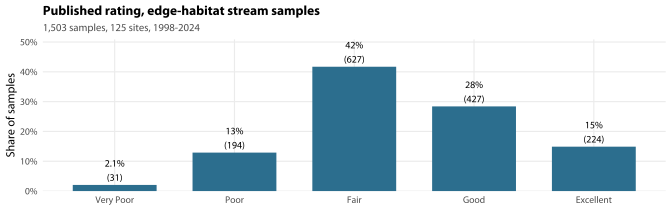
Every rating result in Part III is computed over edge-habitat stream samples that are not empty and carry a rating — 1,503 samples at 125 sites, 1998 to 2024. Is that the population you would want the rating judged on?
Edge only, because riffle sampling stopped in 2007 and the published bands do not apply to riffle samples anyway. Streams only, because wetlands are scored on a different band table and are chapter 11’s. Empty samples carry no rating and are excluded. We chose this set; it is the same one chapters 14, 15 and 16 use, so the comparisons are like for like. If you would rather see the rating judged on a different population — say 2015 onwards, or only the sites you still visit — say so and we will re-run it.
Blocks: Nothing. Recorded so the population behind every figure is explicit. Value: moderate. Costs you: minutes. Refer to it as
dq:rating-analysis-set.
The most quoted number in the report is 38%, and it counts a specific thing. Is that the number you want in front of you?
Of the 160 visits that produced more than one edge sample, 144 produced exactly two, and at 38% of those (95% CI 29-47%, bootstrapped over the 59 sites) the two samples carry different published rating words. Pool in the 16 visits that produced three or four samples and the figure rises to 41%, because “do all the samples agree” is mechanically harder the more samples there are. Both are correct; they answer different questions. We quote the two-sample one throughout because the sentence it supports is about two samples. It is now computed once, in the shared pre-render step, so no chapter can drift from it.
Blocks: Nothing. Recorded because the two figures were previously mixed. Value: moderate. Costs you: minutes. Refer to it as
dq:replicate-discordance-definition.
13.2.2 Questions only you can answer
Which do you want the network to be good at — the network average, or the individual site rating? You cannot have both on the same budget, and nobody has ever been asked to choose.
Priced in Section 13.8, on the roughly 70 stream samples a year the record currently carries. Spend them on 70 sites visited once each and the network mean has a standard error of 0.100 while one site’s rating has 0.543; spend them on 23 sites visited three times and it is 0.148 and 0.314. One rating class is 1.00 score points wide, so the two products move in opposite directions across most of a class. Our first suggestion — a rolling three-year mean — is free and does not make this trade; buying the same reliability inside a single year does, and nobody has been asked which of the two products the network is for.
Refer to it as
dq:monitoring-budget-tradeoff.
Do you want to publish three condition classes, or keep five and print the score with its uncertainty beside the word?
On five classes, a three-sample rating changes the published word 41% of the time, and reaching the protocol’s 20% mark would take about thirteen samples per rating. On three classes the three-sample figure is 23% and the five-sample figure 18%. Neither is comfortable, but five words is the language you have published for a decade and there is a real cost to changing it. Publishing five words off a single sample is not defensible; both of these are. This is suggestion R1b, it is a communication decision about what the public and the councillors are told, and it is yours.
Refer to it as
dq:rating-class-count.
Chapter 12 found two sites that look as though they are in the wrong disturbance tier, in opposite directions. Our headline discrimination result is measured against those tiers — how much weight do you want it to carry?
This is the analytical half of dq:reference-tier-review, which asks the review question itself. What matters for the rating chapters is the size of the effect. Moving 11BMG to reference and dropping 75BKTR raises the headline AUC from 0.76 to 0.84, so both known errors are working against the rating and the result stands — it is understated, not overstated. But relabelling two sites out of 63 moves the figure by 0.08, and dropping any single reference site moves it between 0.74 and 0.80. One creek’s label is worth several hundredths of AUC, which is the same order as the difference between the two rating systems chapter 15 has to choose between. So AUC against these tiers can say that the rating works; it cannot referee a close contest between two ratings, and we have not asked it to.
Refer to it as
dq:tier-errors-calibrate-the-test.
Everything we can test is either a single sample or a ten-year site mean. What you publish is a site-year word. Is there any use of that word we should be evaluating directly?
A ten-year site mean averages away most of the noise, so the discrimination figures in chapter 13 are an upper bound on what the published product achieves rather than an estimate of it. We cannot fix this by re-analysis — a site-year comparison on eleven reference sites would be hopeless — but it changes what the phrase “the rating discriminates well” is entitled to mean. If the site-year word drives a specific decision (a works priority list, a report to councillors), tell us which, and we can test the rating against that use rather than against the tiers.
Refer to it as
dq:rating-grain-mismatch.
13.2.3 What would answer them
Could somebody who knows the creeks — and who has not seen the macroinvertebrate data — rank twenty of them by condition for us?
This is the binding constraint on every discrimination result in the report. Your disturbance tiers were built partly from macroinvertebrate health, so testing a macroinvertebrate index against them is circular; the only non-circular yardstick we have is eleven reference sites. Twenty independent rankings would roughly double the independent information available for testing the rating. An hour or two of an experienced person’s time, done blind.
Refer to it as
dq:expert-creek-rankings.
13.3 The system as published
The system is set out in the June 2025 interim methods document. Four macroinvertebrate measurements are taken from each sample (Table 13.1):
| Factor | What it measures |
|---|---|
| SIGNAL-SF | Mean SIGNAL-SF sensitivity grade of the families present |
| Number of families | Family richness (Council’s FamilyCount) |
| Number of EPT families | Mayfly, stonefly and caddisfly families present |
| % EPT | Percentage of individuals that are mayflies, stoneflies or caddisflies |
Each factor is converted to an integer 0–5 by percentile bands. For streams this is done twice — once against a Blue Mountains urban distribution, once against a reference distribution — giving eight scores, which are averaged. For wetlands a single combined regional-wetland comparison gives four scores. The average is then mapped to one of five words: Very Poor (0–0.99), Poor (1.00–1.99), Fair (2.00–2.99), Good (3.00–3.99), Excellent (4.00–5.00). The band values were set from 2012–2015 percentiles: the top of band 1 is the 20th percentile, band 2 the 40th, band 3 the 60th, band 4 the 80th, and band 5 is everything above.
The implementation used here reproduces all three worked examples in the methods document exactly, and the band table is held as data so that alternative bands can be substituted (apply_health_rating(metrics, bands =)). Getting that far needed one decision that is not in the document, and it is dealt with under band behaviour below (Section 13.5.7).
13.3.1 Can the published bands be regenerated?
Before testing the system, one question about it: can the published bands be regenerated from the databases? The reference column can be. The urban column cannot.
| Comparison | Construction | n | Mean absolute deviation from published |
|---|---|---|---|
| Urban | 2012-2015, urban streams (as documented) | 158 | 3.26 |
| Urban | 2012-2015, urban streams and wetlands | 229 | 2.60 |
| Urban | 2008-2015, urban streams and wetlands (closest fit) | 387 | 1.85 |
| Urban | Whole record, all urban samples | 1770 | 1.89 |
| Reference | 2012-2015, reference streams (as documented) | 43 | 0.84 |
| Reference | 2012-2015, reference streams and wetland | 53 | 1.91 |
| Comparison | Factor | Published | Closest derivation |
|---|---|---|---|
| Urban | SIGNAL-SF | 5, 6.04, 6.51, 7 | 5.67, 6.42, 6.83, 7.25 |
| Urban | Number of families | 8, 11, 14, 18 | 10, 13, 16, 20 |
| Urban | Number of EPT families | 2, 3, 4, 6 | 2, 3, 4, 6 |
| Urban | % EPT | 6.06, 34.62, 58.48, 71.79 | 7.18, 31, 50, 64.97 |
| Reference | SIGNAL-SF | 6.63, 6.92, 7.05, 7.2 | 6.92, 7.18, 7.31, 7.41 |
| Reference | Number of families | 14.6, 16, 17, 18 | 15, 17, 18, 20.6 |
| Reference | Number of EPT families | 4.6, 5, 6, 7 | 4.4, 5, 6, 7 |
| Reference | % EPT | 59.44, 67.05, 76.2, 80.85 | 58.37, 67.59, 73.63, 77.76 |
The reference column reproduces. Its EPT-family boundaries in Table 13.3 come out at 4.4, 5, 6, 7 against a published 4.6, 5, 6, 7 — three of the four exactly, which the chunk above pins — and its % EPT boundaries within 3.09 percentage points on a nought-to-a-hundred scale. Near enough that the documented derivation, 2012–2015 reference-site percentiles, is clearly what was done; and it is the contrast with the urban column, which no window of the database reproduces at all, that carries that conclusion rather than the closeness of any single boundary.
The urban column does not. No window of the database reproduces it (Table 13.2), and the closest fit is not the documented one: it needs a wider window (2008–2015) and the inclusion of urban wetland samples in what the methods document calls “other Blue Mountains urban sites”. Even then the SIGNAL-SF and family-count boundaries remain well below any derivable percentile, and the discrepancies all run the same way — the published urban bands are more lenient than the urban distribution they are said to describe.
Why it matters: the urban comparison is more lenient than it is described as being. If a band set drawn from the 20th–80th percentiles of a distribution is applied to that same distribution, the mean score is 2.5 by construction. The mean urban factor score over the 1,503 samples here is 3.40. The average Blue Mountains creek scores as though it sat near the 70th percentile of Blue Mountains creeks, which is why 85% of samples rate Fair or better. It is also most of why chapter 14’s reset moves as many sites as it does.
The second half of this is a question rather than a finding, and it is on the list: whatever spreadsheet produced Table 1 is not in the material we hold (dq:table1-band-spreadsheet), so the bands cannot be audited and cannot be updated without redoing the work. Generating the table from a script, against a named dataset and a named window, would fix both at once.
13.4 What makes a rating system good
A condition rating is a measuring instrument. Instruments are judged on properties, not on whether their outputs feel right, and the properties are testable. The criteria below are mostly not invented for this report. Three of the four screening properties — discrimination against a known disturbance gradient, reliability on repeat sampling, and non-redundancy between metrics — are Stoddard et al. (2008)’s, who set out five criteria for selecting metrics into a multimetric index and whose responsiveness, repeatability and redundancy tests these are. The fourth, insensitivity to sampling artefact, is ours. It has no counterpart in Stoddard’s five; Hering et al. (2006), the only other place it could have come from, could not be obtained, so it is stated here as the report’s own addition rather than as an established screening test. It earns its place on the evidence in chapter 3 — an uncontrolled change in pick count runs through this record — but a reader should know that its warrant is that evidence and not the literature. The other three are standard (Stoddard et al. 2008), and the discipline of stating them in advance is the main defence against the criticism Suter (1993) levelled at ecological health indices — that combining incommensurable measures into a single number produces something whose meaning cannot be checked. Six apply here. They are the criteria used on the current system in Section 13.5, on the revision in Section 15.4, and written up as a runnable procedure in Section 16.1.
| Criterion | Question | Test |
|---|---|---|
| 1. Discrimination | Does the score separate creeks that are known to differ in condition? | AUC for reference against urban sites; rank correlation with catchment imperviousness. |
| 2. Reliability | Would a repeat sample give the same answer? | Variance components across site, year, visit and replicate; intraclass correlation; probability that a repeat sample changes the published rating word. |
| 3. Independence | Do the factors carry different information, or is the average double-counting one thing? | Correlations among factor scores; effective dimensionality from a principal component analysis. |
| 4. Freedom from artefact | Does the score respond to how the sample was collected and processed rather than to the creek? | Within-site regression of the score on sample abundance and on taxonomic-coverage gaps. |
| 5. Responsiveness | Does the score move when the creek changes? | Within-site response to a known impact; ability to detect a trend. |
| 6. Band behaviour | Are the class boundaries a partition, and are they in sensible places? | Gap, overlap and tie audit (percentile boundaries must be strictly increasing); use of the full 0-5 range; share of samples close to a boundary; share of published ratings that change when the boundaries shift by 0.1. |
AUC, in words, because it is the one number in Table 13.4 that is not self-explanatory and it carries the whole of criterion 1. Take one reference creek and one urban creek at random: the AUC is the chance that the reference one scores the better of the two. 0.5 is a coin toss, because the score is then telling you nothing about which is which, and 1.0 is perfect separation, where the worst reference creek still scores above the best urban one. Everything reported below sits between the two, and the figure reads directly as a percentage of pairs got the right way round.
Two things about these criteria, before the results.
Discrimination and reliability trade off against each other only in appearance. A score that compresses every creek into the middle of its range will look stable on repeat sampling, because there is little range to move within. That is not reliability, it is insensitivity. The scale-free measure — the intraclass correlation, the share of total variance that is between creeks — is the one to compare across systems, and the probability of a rating change should always be read alongside it.
None of these is about whether the rating agrees with expert judgement. That is a seventh, and legitimate, criterion, and it cannot be tested from the databases. Where a statistical criterion and an expert judgement conflict, the honest thing is to report both, and the chapter flags where something is a judgement call rather than a result.
Two of the criteria come with a caveat about the yardstick, not the test, and both are large enough that they belong here rather than in a limitations list at the back. They are Section 13.5.5.2 and Section 13.6.
13.5 Diagnosing the current system
Six criteria, in the order the evidence is strongest. Reliability first, because it is measured directly and it is the finding that decides what the rating can be used for; then the three that describe how the index is built (independence, the double comparison, freedom from artefact); then discrimination, which is the thing the system does well and also the thing with the shakiest yardstick; then responsiveness and band behaviour.
How to read the tests below, and what they are not. This chapter runs on the order of a hundred interval and test statements, and they are not all in the same currency: percentile bootstraps over sites, Wald intervals on mixed-model fixed effects, Satterthwaite and likelihood-ratio p-values, and — for the class-change probabilities — model-based quantities with no interval at all. Each table now says in its caption which currency produced its numbers, and how large the family of tests it belongs to is. Nothing here is corrected for multiplicity, deliberately: these are diagnostics of one system, read together as a pattern, and a false-discovery correction over families this heterogeneous would be a false precision of its own. The consequence is that a single borderline result in this chapter should not be read as a finding on its own — the chapter’s conclusions rest on the several criteria agreeing, and where one turns on a single crossing of a threshold it says so at that point.
13.5.1 Reliability: a repeat sample usually gives a different word
This is the most consequential finding in the chapter, and it can be measured directly rather than modelled, because you have collected replicate samples.
342 samples in the analysis set were collected as two or more edge samples from the same site on the same day — 160 such visits at 65 sites, spread over 1998–2019. These are as close to a true replicate as the archive offers: same creek, same day, same protocol, same field team.
Over the 144 visits that produced exactly two samples, the two fall in different published rating classes 38% of the time (95% CI 29% to 47%, bootstrapped over the 59 sites, because repeat visits to one creek are not independent draws). The median spread in the average factor score between two replicates from one visit is 0.38 points, on a scale where a whole rating class is 1.00 point wide.
That an index inherits substantial noise from the sample is not a surprise, but the external evidence for it is thinner than this report previously claimed, and the honest version is worth stating. Ostermiller and Hawkins (2004) found RIVPACS-type assessments robust to both collection method and subsampling effort on average; what moved sites between condition classes in their study was which predictive model was used, and their recommendation is a design prescription rather than “quantify and report sampling error beside the index”. So the reliability criterion here is not carrying external backing for replicate-to-replicate variation in a multimetric score — the evidence for it is the number above, computed from your own repeat samples, which is stronger than a citation would have been. What you have, and most programs do not, is the replicate data to measure it rather than assume it.
Two qualifications belong beside that number, because it is quoted more often than any other in this report.
| Rating class of the visit mean | Visits | Replicates disagree | Median spread |
|---|---|---|---|
| Very Poor | 1 | 100% | 0.25 |
| Poor | 39 | 59% | 0.62 |
| Fair | 74 | 36% | 0.38 |
| Good | 35 | 34% | 0.25 |
| Excellent | 11 | 18% | 0.12 |
First, discordance runs from 59% at visits rated Poor down to 18% at visits rated Excellent. Table 13.5 also carries a Very Poor row, discordant at 100% on 1 visit — too few to read as a rate, which is why the range is quoted from Poor down. It is driven almost entirely by how close the creek sits to a class boundary rather than by how noisy the sample is: a logistic regression of discordance on distance to the nearest boundary gives a coefficient of -8.6 (z = -5.9). A creek sitting mid-class is far better measured than 38% implies, and one sitting near a boundary is far worse.
Second, the figure depends on how many samples the visit produced, so be exact about which one is quoted. 16 of the 160 replicate visits produced three or four samples, and “do all the samples at this visit agree” is mechanically harder to satisfy the more samples there are: 38% over the 144 two-sample visits against 62% over the 16 with more, and 41% if you pool all 160. This chapter quotes the two-sample figure throughout, because the sentence it supports is about two samples. The pooled 41% answers a different question and should not be substituted for it.
| Level | Variance | Share of total | Standard deviation |
|---|---|---|---|
| Between sites | 0.410 | 49% | 0.641 |
| Between years | 0.131 | 16% | 0.361 |
| Between visits to the same site | 0.115 | 14% | 0.339 |
| Between replicates within a visit | 0.183 | 22% | 0.428 |
Only 49% of the variance in the published score is between creeks (Table 13.6). 16% is which year the sample happened to be taken in — the weather, the field crew and the laboratory’s practice that season, a component shared by every creek in the network — and the remaining 36% is the same creek differing from itself within a year: 14% between visits and 22% between replicate samples taken at the same visit.
Separating the year matters. Without it the between-creek share comes out at 58% rather than 49%, because a wet year that lifts every creek in the network gets charged to the individual creeks. It matters again in Section 13.5.6, where it decides the answer.
The within-visit standard deviation is 0.43 points and the within-site standard deviation — everything that is not a stable property of the creek — is 0.65 points.
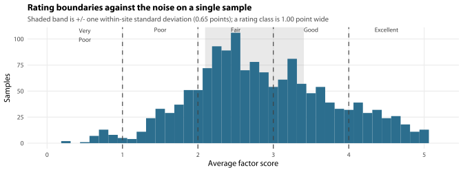
Put those two facts together. Rating classes are 1.00 point wide and the noise on a single sample is 0.65 points. The classes are narrower than the measurement error. That one sentence is most of this chapter.
| Basis of the published rating | Probability the class changes | 95% interval |
|---|---|---|
| One sample, re-sampled the same day (replicate error only) | 45% | 42% to 49% |
| One sample, re-sampled at another visit (current practice) | 60% | 57% to 63% |
| Mean of three samples over a rolling three-year window | 41% | 38% to 44% |
| Mean of five samples | 32% | 29% to 36% |
| Mean of 13 samples | 19% | — |
The two ways of asking are consistent, and the model sits at the pessimistic end of what the replicates show. The fitted probability that two same-day replicates differ in class is 45%; the observed figure across 144 two-sample replicate visits is 38% (95% CI 29% to 47%), so the fitted figure falls inside that interval and the replicates do not refute it — but it is 7.2 percentage points higher than the direct count. It is the modelled figure that is quoted onward, not the observed one. 60%, 41%, the 13-sample figure in Table 13.7 and the class-count grid of Section 13.7 are all functions of the same fitted variance components. Each now carries a 95% interval from a 1000-replicate parametric bootstrap of that fit — 57% to 63% and 38% to 44% respectively, and 10 to 20 samples for the last — and those intervals are the right measure of how precisely the model determines them. They are not a measure of whether the model is right. The same-day comparison above is that question, and it puts the model at the unfavourable end of what the replicates show; read these figures as the unfavourable end of a range whose favourable end is the direct replicate count.
Plain reading. Sample a creek twice and publish both results, and the two carry different words roughly two times in five. That is not a criticism of the field or laboratory work — it is what natural variation in a macroinvertebrate sample does. It means a single sample cannot support a five-class published rating, and that year-on-year movement in a site’s rating is mostly noise. The remedy is not a coarser index; it is to publish the rating from more than one sample. Three cut the probability to 41%. That is a large improvement and it is not a cure: the criterion this report sets for itself in Section 16.1 is a class-change probability below 20%, and on five classes reaching it needs about 13 samples — anywhere from 10 to 20 once the uncertainty in the fit is carried. Which raises the question of how many words the data can carry, and Section 13.7 answers it.
13.5.2 Independence: eight scores carry about three dimensions
| SIGNAL-SF | Number of families | Number of EPT families | % EPT | |
|---|---|---|---|---|
| SIGNAL-SF | 1.00 | -0.11 | 0.43 | 0.43 |
| Number of families | -0.11 | 1.00 | 0.59 | 0.19 |
| Number of EPT families | 0.43 | 0.59 | 1.00 | 0.53 |
| % EPT | 0.43 | 0.19 | 0.53 | 1.00 |
The four factors are not four independent readings (Table 13.8). Number of EPT families correlates 0.59 with number of families and 0.53 with % EPT — it is partly a richness measure and partly an EPT abundance measure. SIGNAL-SF correlates -0.11 with family count, which is to say negatively: samples with more families have slightly lower mean sensitivity, because the extra families are tolerant ones. On a principal component analysis of the four raw factors, the first two components carry 85% of the variance and the effective dimensionality is 2.5.
Across all eight stream scores the effective dimensionality is 3.1 and the first two components carry 76%. So eight numbers are averaged to express about three independent facts about the sample. That is not fatal — averaging correlated indicators is a legitimate way to reduce noise — but it does mean the equal weighting is not what it appears. Because EPT family count sits between richness and EPT abundance, the EPT signal enters the average roughly two and a half times and sensitivity roughly once.
13.5.3 The double comparison: the reference scoring adds almost nothing
Streams are scored twice, against urban and against reference distributions, and the eight results averaged. Nobody appears to have asked whether the second comparison adds information.
The urban composite and the reference composite correlate at 0.89 (Pearson) across 1,503 samples. Rescaled to the same mean and spread, the urban composite alone reproduces the published rating class for 82% of samples and is never more than one class away (100%); Kendall’s tau between the urban composite and the published average is 0.92.
Worse, the reference comparison does its shifting with very little resolution, because the reference bands were drawn from a narrow distribution and band 1 is therefore enormous. Reference band 1 for % EPT runs from 0.01 to 59.44 — from a sample with almost no mayflies to one where three individuals in five is a mayfly.
| Factor | Reference band 1 range | Share of samples scoring exactly 1 |
|---|---|---|
| SIGNAL-SF | 4.51-6.63 | 29% |
| Number of families | 3.00-14.60 | 43% |
| Number of EPT families | 0.01-4.60 | 57% |
| % EPT | 0.01-59.44 | 62% |
62% of samples score exactly 1 on the reference % EPT factor and 57% on reference EPT families (Table 13.9). Those two factors are, for most of the network, constants. Averaging in two near-constant columns adds four numbers to the mean without adding information: the published average and the urban composite alone have almost identical spread (0.93 against 0.92) and rank the network almost identically (Kendall’s tau 0.92). The reference comparison shifts the level; it does not change the order and it does not add resolution. Be precise about this, because it would be easy to write that the doubling compresses the scale, and it does not: the reference composite on its own is the most spread out of the three (0.99). The defect is redundancy, not compression.
The reference distribution is nonetheless the right benchmark for saying what “Excellent” means, so the fix is not to throw it away. Use it as an anchor rather than as a second score: one score per factor, running from a degraded anchor drawn from the urban distribution to a reference anchor drawn from the reference distribution. That uses both benchmarks, halves the number of numbers and doubles the resolution. Chapter 15 builds it (Section 15.3, rule 3) and chapter 14 shows why it has to come with the band reset rather than after it — resetting the bands alone makes two of the reference columns less informative than they are now (Section 14.4.2).
13.5.4 Freedom from artefact: two factors measure laboratory effort
This is the mechanism behind most of what chapter 15 suggests changing.
The premise is chapter 3’s (Section 3.4) and it is not in dispute: the laboratory is processing roughly twice as many animals per sample as it was in the 2000s, and once the count is held fixed and a strict family list is used, family richness shows no net trend across the record (0.05 families per decade, -0.39 to 0.50) — and over 2010–2024 it falls, -0.85 (-1.65 to -0.05), on an interval that excludes zero. Two of the four rating factors are counts of families. Here is what that does to the rating.
| Measure | Between sites | Within a site | Site and year (95% CI) |
|---|---|---|---|
| Published average factor score | +0.67 | +0.46 | +0.43 (+0.38 to +0.49) |
| SIGNAL-SF score | -0.04 | -0.07 | -0.07 (-0.13 to -0.01) |
| Number-of-families score | +0.87 | +0.71 | +0.75 (+0.70 to +0.81) |
| Number-of-EPT-families score | +0.60 | +0.39 | +0.38 (+0.32 to +0.44) |
| % EPT score | +0.47 | +0.29 | +0.27 (+0.21 to +0.34) |
Two units are in play here. Table 13.10 is in standard deviations, so that four scores on four different scales can be compared with one another; every sentence below it is in published score points, from separate unstandardised fits on the same samples. A figure taken from the table and a figure taken from the prose are not comparable even when they print the same digits, which at present two of them do.
Within a site, a sample with 2.7 times as many individuals in it scores 0.43 points higher on the published average. Across the interquartile range of sample abundance here — 79 to 206 animals — the published score moves 0.41 points (0.36 to 0.46), 41% of a full rating class, with no change in the creek. Compared across creeks — which is what a reader of the published number is actually doing — the same interquartile range carries 0.60 points, but that larger figure also contains the real difference between a productive creek and an unproductive one and is not a within-creek estimate of the artefact. The number-of-families score is the worst of the four at +0.71 standard deviations per log unit; % EPT, being a proportion, is the most resistant and is not immune (chapter 3 puts a number on how far from immune: Section 3.4.4). Adding the year term changes almost nothing — the composite goes from +0.46 to +0.43 — so this is not a trend in disguise.
Neither database records a subsampling protocol or a pick count, so whether the abundance change is procedural or ecological cannot be settled from the data (dq:pick-count-protocol). That is precisely why the rating should not depend on it. Chapter 15 shows what the same coefficients look like when the two count factors are standardised to a fixed depth of 20 individuals — the rating chapters’ depth, which differs from the 50 used in the trend chapters for the reason Section 3.4.3.3 sets out.
A second artefact affects SIGNAL-SF specifically. It has no grade for 91 of 233 recorded taxon names, and the share of individuals in a sample with no grade drifts from about a fifth in the 2000s to two fifths in 2014 and about a quarter now (chapter 1). Within a site, the published score moves -0.07 standard deviations for every 10 percentage points of ungraded individuals. The effect on the composite is small, but it is an effect of laboratory practice on a published environmental indicator and it has no business being there.
There is a third channel and it is not a laboratory one: the rating is lower on visits where the creek was not flowing, by about a third of a standard deviation. It is set out under responsiveness, where the flow tests live (Section 13.5.6.2), because that is where it was found — but it is a freedom-from-artefact result, and it is the one channel of the three that chapter 15’s revision was never tested against until now.
13.5.5 Discrimination: the composite works, but not through SIGNAL-SF
| Measure | AUC reference vs urban | AUC reference + slightly disturbed vs urban | Rank correlation with imperviousness |
|---|---|---|---|
| Published average factor score | 0.76 (0.59-0.90) | 0.87 (0.79-0.95) | -0.57 |
| SIGNAL-SF | 0.65 (0.49-0.79) | 0.70 (0.59-0.81) | -0.21 |
| Number of families | 0.57 (0.39-0.75) | 0.72 (0.61-0.83) | -0.42 |
| Number of EPT families | 0.77 (0.64-0.88) | 0.86 (0.78-0.94) | -0.54 |
| % EPT | 0.75 (0.57-0.89) | 0.83 (0.74-0.92) | -0.52 |
The composite discriminates. Site mean scores separate reference from urban sites with an AUC of 0.76 and reference plus slightly disturbed from urban at 0.87, and correlate -0.57 with total catchment imperviousness. In the terms of Section 13.4, the first of those figures says the composite puts a randomly drawn reference-and-urban pair the right way round 76% of the time. For a four-number index built by hand that is a good result, and it is the main thing the current system has going for it. Two caveats attach to it, and the second is large.
Where the discrimination comes from. The two EPT factors carry it. SIGNAL-SF is the weakest of the four on the good-condition comparison (0.70) and on imperviousness (-0.21, close to nothing), though on reference against urban the raw family count is weaker still (0.57 against 0.65). On 11 reference sites the single-factor intervals overlap heavily — read Table 13.11, not the point estimates — so the ordering is indicative. What is solid is that SIGNAL-SF carries almost no relationship with imperviousness, which is the one yardstick here that is not partly your own judgement. The sensitivity factor, conceptually the heart of a macroinvertebrate index, is contributing almost nothing in this network.
Chapter 8 explains why, and it is not the missing grades. It is scale compression: across the families whose occurrence changed over the record, SIGNAL 2 explains 22% of the between-family variation in occupancy trend (0.130 per grade, p = 0.00002) where SIGNAL-SF explains 5.7% (0.077 per grade, p = 0.04), and in a joint model SIGNAL-SF falls to −0.049 (p = 0.28) — it adds nothing once SIGNAL 2 is in. SIGNAL-SF grades Culicidae 6 where SIGNAL 2 grades it 1, Dytiscidae 7 against 2, Veliidae 7 against 3. The tolerant families that are disappearing from Blue Mountains creeks are scored by SIGNAL-SF as clean-water animals, so their disappearance barely moves the index.
13.5.5.1 The yardstick has known errors in it, and they matter more than the result
The tiers are not a measurement. They are a classification, 11 reference sites against 52 urban ones here, and chapter 12 found at least one site in the wrong bucket in each direction.
11BMGis tiered urban. The one archive site that passes chapter 12’s stream-type test sits 924 m from it, and AUSRIVAS scored that site band A on 18 of 23 runs. Your own 17 edge samples at11BMGaverage 4.24, and its catchment is 1.2% impervious against a reference median of 0.0% and a reference maximum of 1.9%.75BKTRis tiered reference, and two independent lines of evidence call the assemblage there impaired — AUSRIVAS band B, significantly impaired, on all four nearby archive runs, and your own samples, which score it 2.48 (Section 12.5). The two systems agree with each other and disagree with the tier, which is the point: the designation is a catchment attribute (protected special area, very low imperviousness) and the bands are percentiles of assemblages. The two come apart, and the published bands inherit the gap.
Neither is a mistake anyone should feel bad about — and note that “reference” does not name one set of creeks in this book either. Chapter 12 counts five defensible answers (Section 12.3); the 11 used here is the one Part III leans on. What matters is what the errors do to the test.
| Reference set | Reference sites | AUC, reference against urban (95% CI) |
|---|---|---|
| As tiered | 11 | 0.76 (0.59-0.90) |
| 11BMG moved to reference | 12 | 0.79 (0.63-0.93) |
| 75BKTR dropped | 10 | 0.80 (0.65-0.93) |
| Both | 11 | 0.84 (0.70-0.94) |
Both known errors work against the rating, so correcting them raises the result rather than lowering it — from 0.76 to 0.84 (Table 13.12). The discrimination finding survives, and if anything Table 13.11 understates it.
The useful part is the size of the movement. Relabelling two sites out of 63 moves the AUC by 0.08. Dropping any single reference site moves it anywhere from 0.74 to 0.80; dropping any single urban site moves it between 0.75 and 0.77. So one creek’s classification is worth several hundredths of AUC, which is the same order as the difference between whole rating systems that chapter 15 has to arbitrate. AUC against these tiers can say that the rating works. It cannot referee a close contest between two ratings, and any comparison that turns on a few hundredths should be read with that in front of it.
Two things would help, and only one of them is analysis. Reviewing the tier assignments is on the list as dq:reference-tier-review; an independent set of creek rankings from somebody who knows the creeks and has not seen the macroinvertebrate data is dq:expert-creek-rankings, and on value against what it would cost you it is one of four items tied at the top of this chapter’s list. It prints as the last of the seven above: inside a tie the order is alphabetical by id, not a ruling on which of them matters most, and which to commission first is a judgement for you rather than one this report can make for you.
13.5.5.2 The tiers are partly built from the thing being tested
There is a deeper version of the same problem, and it does not go away with better bookkeeping. The reference and slightly disturbed sets come from methods Appendix 2, which used, among other criteria, “consistently good–excellent macroinvertebrate health”. Testing a macroinvertebrate index against a classification partly built from macroinvertebrate health is circular, and the degree of circularity is unknown because the derivation is not recorded (dq:appendix2-dci-method).
This is why imperviousness is run alongside in Table 13.11 and Table 13.12: it is independent of the biology. It is also modelled rather than measured (chapter 4), so it is not a clean substitute — it trades one weakness for another. This is not a local failing. Chessman (2021) makes the same criticism of AUSRIVAS itself, along with the related point that reference condition is treated as fixed when catchments and climate are not.
What follows for how the discrimination number should be read: it is a statement of agreement between the index and your tiering, not of accuracy. That is still worth having — a rating that disagreed with the tiering would be a serious finding — but it is a weaker claim than it looks, and it is the reason this chapter does not lean on discrimination when it says what the rating is good for.
13.5.6 Responsiveness
The archive supports three tests, and they do not agree. Catchment fire moves the rating in the expected direction once the sampling year is allowed for; whether that movement is established is a question about how few creeks in the record have ever burnt, and it is measured below rather than assumed. The one designed control–impact pair points the right way but cannot carry a statistical test. And flow state — a physical variable that demonstrably moves both the water chemistry and the community composition — does not move the rating up or down its scale, but it does something less comfortable: samples taken when the creek was not flowing score lower than samples taken when it was. That is a property of the visit rather than of the creek, so it belongs with Section 13.5.4 as much as it belongs here.
Catchment fire. Comparing samples taken where more than half the catchment burnt in the previous three years against samples at the same sites otherwise, and separating out the sampling year, the published score falls by 0.19 points (95% CI 0.01 to 0.37; 940 samples, 64 of them post-fire, 83 sites). Treating burn extent as continuous rather than as a threshold gives -0.28 points for a fully burnt catchment (-0.48 to -0.08).
That interval is fitted at the sample and the quantity does not live there. Burn extent is a property of the catchment inside a three-year window, so it varies at the site-year: those 940 rows are 773 site-years, and only 14 of the 83 sites are ever burnt. It is not the defect chapter 4 was found to have — here burn status varies more within a creek (SD 0.19) than between creeks (SD 0.13), no creek is burnt throughout, and every burnt sample sits at a creek that also holds unburnt samples, so this is a before-and-after and not a comparison of creeks that happen to differ. What it does share is the denominator. Refitted on the site-year means the fall is 0.16 points (-0.02 to 0.35), an interval that covers zero; and a site permutation — each burnt catchment’s burnt years moved as a block onto a creek sampled in those same years, 1,200 times, with the null’s spread held to the fitted standard error — puts the estimate at p = 0.083. The direction is consistent — samples from burnt catchments score lower on every fit here — but a response to catchment fire is not established on these data. With 14 burnt catchments in the record this is a comparison of 14 creeks, and the sample-level interval is the one the archive most easily produces and the one it is least entitled to.
A note on the two fire sets, because two chapters report this test. The 940 samples here are every edge sample in the analysis set with a burn-extent covariate against it from 2010 on. Section 15.4.1 runs the same contrast on the same instrument but over a slightly smaller set — the samples every candidate system can rate, which drops the ones the revision cannot rarefy (Section 15.3.4) — so its sample and site-year counts are a little lower than these and its permutation p is a little different. Neither figure is a restatement of the other, and the permutation is a Monte Carlo estimate from 1,200 draws in both places, so the last digit of either is draw noise. The adjudication is the same on both sets.
The estimate is also sensitive to how the sampling years are handled, and it is instructive to see how much. Without a year random effect the same comparison gives -0.10 points (-0.28 to 0.08) — an interval spanning zero, from which the only available conclusion is that nothing was established. The burnt samples are not one fire: 34 of the 64 fall in 2014–2017 and 30 in 2020–2024. The years they fall in sit +0.04 points from the mean of the network’s own unburnt samples — too little for the year term to be removing a network-wide rise from under the burnt sites. What it removes is the year-to-year movement those two windows happen to sit on, and a comparison of 14 creeks is at the mercy of it.
The result is reported here even though it favours the incumbent: the revised score of chapter 15 responds less to fire, and with a larger standard error (Section 15.4.1). Chapter 4 takes the fire question further and finds that burn severity beats burn extent as a predictor, which is a better covariate than the threshold used here.
13.5.6.1 A known point impact
You established site 88GHZ as an impact site and 87GHZ as its control after the bifenthrin contamination incident at Hazelbrook in 2023. Three paired visits exist.
| Site | Date | SIGNAL-SF | Families | EPT families | % EPT | Score | Rating |
|---|---|---|---|---|---|---|---|
| 87GHZ (control) | 29 Aug 2023 | 6.75 | 18 | 4 | 14.6 | 2.62 | Fair |
| 88GHZ (impact) | 29 Aug 2023 | 8.20 | 9 | 2 | 35.0 | 2.38 | Fair |
| 87GHZ (control) | 07 Nov 2023 | 6.84 | 23 | 5 | 38.5 | 3.25 | Good |
| 88GHZ (impact) | 07 Nov 2023 | 5.30 | 14 | 2 | 2.9 | 1.38 | Poor |
| 87GHZ (control) | 16 Apr 2024 | 7.00 | 9 | 4 | 34.6 | 2.12 | Fair |
| 88GHZ (impact) | 16 Apr 2024 | 6.00 | 16 | 3 | 29.3 | 1.88 | Poor |
The rating puts the impact site below its control at every visit (Table 13.13), by 0.79 points on average. Three pairs cannot carry a statistical test, but as a sanity check the system behaves as it should on the only impact comparison the site register itself sets up as one. Two cautions. The separation is a separation of class at only two of the three visits — both sites rate Fair in August 2023 — and the archive holds no pre-incident sample at either location, so this is a control–impact comparison without a “before” and cannot separate the incident from a pre-existing difference between the two creeks. They are two creeks: the delineation gives the control 49.2 ha and the impact site 36.0 ha, and the two catchments do not overlap at all, so the difference the table shows is a difference between catchments and not a difference within one. One pre-incident sample at either location would turn it into a design that can carry a test, and one may exist under an older site code — that is the ask (dq:hazelbrook-pre2023).
It is the only such pair Council set up deliberately, and the archive’s other control–impact set — the 2012 Jamison Creek contamination (chapter 17) — is missing its “before” in the same way, so neither can carry the test. There is no before-and-after data for the stormwater treatment works in a form that can be analysed (chapter 17), and building that would do more for the credibility of the rating than any change to its arithmetic.
13.5.6.2 Flow state
How much water is moving past the officer is the strongest single visit-level predictor of water chemistry in the record: one step up the six-level flow-state scale adds nearly three percentage points of dissolved oxygen saturation (Section 6.7). The same variable moves the community composition, on 921 edge stream samples (Section 9.6.1). Both effects are real and both are physical. The rating tracks neither of them up the scale — but it is not indifferent to flow either, and the difference between those two statements is the whole of this section.
| Rating input | n | Change per step up the flow scale (95% CI) | p (linear) | p (six levels) |
|---|---|---|---|---|
| Published score (average of eight factors) | 921 | 0.000 (-0.039 to 0.039) | 0.99 | 0.02 |
| SIGNAL-SF | 921 | +0.019 (-0.007 to 0.045) | 0.15 | 0.06 |
| Family count | 921 | -0.155 (-0.422 to 0.111) | 0.25 | 0.15 |
| EPT family count | 921 | +0.004 (-0.097 to 0.105) | 0.94 | 0.16 |
| % EPT | 921 | +0.014 (-1.111 to 1.139) | 0.98 | 0.75 |
The scale is ordered, not numeric, and forcing a straight line through it is what hides the response. Free the six levels — the last column of Table 13.14 — and the composite separates them: \(\chi^2\) = 13.90 on 5 degrees of freedom, p = 0.02. The shape is not a slope, it is a step: every level from low upwards sits above no flow, none of them is distinguishable from the others, and no flow sits below all of them.
The rating does not track flow state, but it is depressed by sampling a creek that is not flowing. There is no monotone response across the six-point scale — 0.000 points per step, p = 0.99. But samples taken at no flow score 0.28 points lower than samples at any other flow state (95% CI 0.08 to 0.49 points lower; 39 samples at 19 sites, 18 of which also hold flowing samples, spread over 2009–2023), and SIGNAL-SF, the family count and the EPT family count all fall with it. That is 0.32 standard deviations — larger than the rating’s response to catchment fire — and it is a property of the visit rather than of the creek.
Three things about that number. It is not one dry creek or one drought year: 18 of the 19 sites with a no-flow sample also hold flowing samples, so the comparison is largely within creeks. It is not one model — site fixed effects, dropping the year term and adding a month term give -0.26, -0.31 and -0.31. And it is not a curve: adding a quadratic term in flow level buys nothing (p = 0.98), and dropping the no-flow visits leaves the remaining five levels indistinguishable (p = 0.18). That is what a step looks like.
Three of the four inputs move with the composite, so this is not an artefact of the averaging: SIGNAL-SF -0.20 (-0.34 to -0.05), the family count -1.37 (-2.75 to 0.00) and EPT families -0.63 (-1.16 to -0.11). % EPT, a proportion, does not.
Whether a creek is flowing on the morning an officer arrives is a sampling condition, not a property of the creek’s health, so a rating that drops 0.28 points on those visits is failing the freedom-from- artefact test of Section 13.5.4 through a second channel — one nothing in this report had looked for. It is the same defect as the effort sensitivity, and it is of much the same size: the published rating responds more to whether the creek happened to be flowing on the day than to whether half its catchment burnt in the previous three years (-0.21 standard deviations, Section 13.5.6 above, and that fire estimate is the one that does not survive being refitted at the site-year). Chapter 15 asks whether the revised score inherits it (Section 15.4.1.2).
One caution in the other direction. Thirty-nine samples is not many, and a dry-creek visit could be picking up a real short-term ecological response rather than a sampling artefact — a pool that has stopped flowing genuinely holds fewer EPT families. Flow state here is an officer’s field judgement recovered from a free-text box (Section 9.3.3), not a measurement. A stage or discharge reading at the time of sampling would separate the two, and they have opposite implications for the rating.
Put the three responsiveness tests together and the pattern is the same one the rest of the chapter keeps finding. The rating moves with laboratory effort, which it should not (Section 13.5.4); it moves with catchment fire only once the sampling year is separated out, and not once the comparison is refitted at the catchment, where it is a comparison of only 14 creeks; and it does not track a physical driver that measurably reorganises the community, while still being pulled down by the one state of that driver a field officer cannot choose. A composite that is stable against the things it should follow and unstable against the things it should ignore is not robust — it is coarse in the wrong places.
13.5.7 Band behaviour
Three things are wrong with the bands and one is right.
Right: the 0 band is not percentile-based, and should not be. A sample with no EPT families at all is qualitatively different from one with few, and giving it a floor of zero is correct.
Wrong, first: the tables are not a partition, so some values fall in no band at all. The urban SIGNAL-SF column runs 4.50–5.00 for a score of 1 and 5.01–6.04 for a score of 2, so a mean SIGNAL-SF of 5.004 has nowhere to go. The reference SIGNAL-SF column has the same gap between 4.50 and 4.51, and the pattern recurs wherever the next band begins at x.01. There is a matching overlap in the wetland family-count column (chapter 11). This report resolves it with a stated rule — a value in a gap takes the score of the band below — which is conservative and matches how a reader would interpret the table, but it is a decision we made, not a reading of the document. A published system should not need one, and generating the table from code with an assertion that the four boundaries are strictly increasing would remove the possibility.
Wrong, second: the factor scores do not use their range evenly.
| Comparison | Factor | 0 | 1 | 2 | 3 | 4 | 5 |
|---|---|---|---|---|---|---|---|
| Urban | SIGNAL-SF | 0.1% | 0.7% | 9.3% | 14% | 31% | 46% |
| Urban | Number of families | 0.1% | 6.9% | 15% | 21% | 28% | 29% |
| Urban | Number of EPT families | 2.6% | 22% | 18% | 16% | 26% | 15% |
| Urban | % EPT | 2.6% | 5.9% | 25% | 30% | 19% | 17% |
| Reference | SIGNAL-SF | 0.1% | 29% | 17% | 8.6% | 9.9% | 35% |
| Reference | Number of families | 0.1% | 43% | 15% | 6.4% | 7.1% | 29% |
| Reference | Number of EPT families | 2.6% | 57% | 15% | 10% | 6.1% | 9.0% |
| Reference | % EPT | 2.6% | 62% | 12% | 12% | 5.5% | 5.8% |
76% of samples score 4 or 5 on urban SIGNAL-SF, and 65% score 0 or 1 on reference % EPT (Table 13.15). The two have different causes and only one is a defect. A percentile-banded factor applied to the population it was drawn from should put about a fifth of samples in each band, and urban SIGNAL-SF does not — that is the leniency of Section 13.3.1 showing up in the scores, and Section 14.4.2 shows the reset fixing it. The reference bands are a different matter. They are drawn from reference sites and applied to a mostly urban network, so a pile-up at band 1 is the design working, not a reproducibility failure — and because the re-derived reference bands turn out to be more demanding than the published ones, resetting them makes the pile-up worse rather than better (Section 14.4.2). What is wrong with the reference column is not the pile-up but the resolution: a band 1 running from 0.01 to 59.44 % EPT cannot distinguish a dead creek from a fair one.
Wrong, third: the discretisation into integers throws away information for no benefit. The average of eight integers can take only 38 distinct values in practice, and 9.4% of samples sit within 0.125 points of a rating boundary — one eighth of one score point, which is a single factor moving by one band. Given a within-site standard deviation of 0.65 points, samples near a boundary are effectively unclassified.
13.6 Every criterion above is tested at the wrong grain
One thing applies to all six criteria and it is easy to miss. Everything in this chapter is evaluated either at the sample grain or at the ten-year site mean grain. The product you publish is neither: it is a site-year word.
Nothing here evaluates that object directly, and the direction of the error is knowable. Discrimination in particular would be weaker at the site-year grain than at the ten-year mean, because a site-year mean rests on one or two samples rather than ten, and averaging ten samples removes most of the noise Section 13.5.1 measures. So the AUC figures above are an upper bound on what the published product achieves, not an estimate of it.
This is not a flaw in the tests — a site-year AUC on 11 reference sites would be hopeless — but it is a reason to be careful about the sentence “the rating discriminates well”. It discriminates well between creeks, averaged over a decade. That is the claim the evidence supports, and it is the claim Section 13.9 makes.
13.7 How many rating classes can the data support?
Section 16.1 prescribes “publish fewer classes” as the remedy for boundary sensitivity, so it ought to say how many fewer. The fitted variance components answer it directly. Holding the 0–5 scale fixed and cutting it into equal classes:
| Classes | Class width | One sample | Mean of three | Mean of five |
|---|---|---|---|---|
| 2 | 2.50 | 33% (28-36) | 23% (18-26) | 19% (14-22) |
| 3 | 1.67 | 41% (38-44) | 23% (21-28) | 18% (16-22) |
| 4 | 1.25 | 52% (49-55) | 35% (30-37) | 28% (23-30) |
| 5 | 1.00 | 60% (57-63) | 41% (38-44) | 32% (29-36) |
Three classes beat five by a wide margin at every sample size: 23% (21-28) on a rolling three-year window against 41% (38-44), and 18% (16-22) on five samples against 32% (29-36). They are not distinguishable from two — the two intervals overlap over almost their whole length — which is itself useful — collapsing to a two-word rating buys nothing over a three-word one and loses a word. (Two classes look better on a single sample only because one cut can be wrong at most half the time.) No scheme reaches 20% on three samples; three classes on five samples does.
How much of that turns on the interval. Each cell now carries one, so the question can be asked properly rather than left open. On three samples one of the four has an interval reaching below the 20% line — the two-class scheme, whose lower limit is 18% — so that is the one scheme that sampling error alone could carry under the criterion, and none reaches it on the point estimate. Three classes on five samples sits under the line at 18%, on an interval of 16% to 22%, which straddles it.
That grid inherits the uncertainty Section 13.5.1 left on the table, and the interval in each cell is not a measure of it. Every figure in the grid is a function of the same fitted 0.65-point within-site standard deviation; the brackets say how precisely the model pins each cell down, and the one direct check available — the replicate count of 38% against a modelled 45% — says the model itself sits at the pessimistic end, which no bootstrap of that model can see. The ranking of the schemes is not in doubt and five classes is too many on any reading, but the sentence above turns on a single crossing of the 20% line, and a noise term recalibrated to the replicates would move it further than sampling error does. Read it as the strict version of the finding, not as a measurement.
One caveat on the arithmetic. It counts the year effect as noise, because a network-wide wet-year rise moves a creek’s published word without the creek changing in any way you can act on. On the opposite view — that a year’s weather is part of what the word should describe — the noise term would be the within-year standard deviation of 0.55 rather than 0.65 points, and every figure in Table 13.16 would be lower. The ranking of the schemes would not change, and neither would the conclusion that five is too many.
What this means for the published word. Five words on one sample is the current product and the data do not support it. Five words on three years of samples is a large improvement and still misses the criterion by a factor of 2.0. Three words on a rolling three-year window is the combination these data come closest to supporting, and three words on five samples meets the criterion outright. If you want to keep five words for continuity — a legitimate communication choice, and the reason this is a question on the list rather than a suggestion (
dq:rating-class-count) — then the score and an uncertainty band need to go beside them, so a reader can see when a creek is sitting on a boundary and the word is arbitrary. The 59% discordance among visits rated Poor is what that looks like in practice.
13.8 Where the next monitoring dollar goes
Everything above says the published rating needs more than one sample behind it. This section says what that costs, because the money you spend on more sites and the money you spend on more visits buy different products, and you cannot have both.
Samples spent column. Variance components fitted on the 1,503 stream edge samples of the analysis set, 125 sites in the 27 calendar years from 1998 to 2024: creeks differ from each other with a standard deviation of 0.64, a year shifts the whole network by 0.37, and repeat visits to the same site in the same year differ by 0.54. One rating class is 1.00 score points wide. The two right-hand columns move in opposite directions and that is the entire finding. Currency: analytic standard errors derived from the fitted variance components, with no interval on the components themselves; they are exact arithmetic on estimated quantities, not measurements.
| Sites | Visits per site | Samples spent | Standard error of the network mean | Standard error of one site’s rating |
|---|---|---|---|---|
| 70 | 1 | 70 | 0.100 | 0.543 |
| 35 | 2 | 70 | 0.126 | 0.384 |
| 23 | 3 | 69 | 0.148 | 0.314 |
| 17 | 4 | 68 | 0.168 | 0.272 |
Read the two right-hand columns against each other. Spending the same 70 samples on 70 sites once each gives the tightest possible estimate of how the network is doing — standard error 0.100 — and the worst possible estimate of how any one creek is doing, because a single visit carries 0.543 score points of noise, more than half of the 1.00 score points a rating class is wide. Splitting the budget across 23 sites visited three times — 69 samples, since sites have to be whole — reverses it: the site rating tightens to 0.314, and the network mean loosens to 0.148.
So the reliability fix comes in two forms and only one of them costs money. The rolling three-year mean suggested in Section 13.9.1 is the free one: it averages samples you already collect, and what it costs is the ability to say anything about a single year. It is also the better buy against a site’s long-run condition — three visits spread over three years carry 0.378 score points of error against 0.482 for three visits inside one year. Buying the same reliability with money instead — fewer sites, visited more often, in the same year — is the version that costs you the network trend, and nothing else in the report says so.
Current practice is the top row of Table 13.17: about 70 stream samples a year carrying a usable rating, mostly one visit per site. That is a choice nobody has made explicitly. It might well be the right one. It is worth making on purpose, and it is yours to make rather than ours (dq:monitoring-budget-tradeoff).
Two things this arithmetic does not cover, and both would change the answer:
- A cheaper laboratory protocol — a smaller pick, or fewer rating factors — is a third way to spend the money and nothing in this report has costed it. The four rating factors are strongly correlated (Section 13.5.2), so a reduced set may reproduce the full rating closely enough to free real money. That is a few days’ work and nobody has done it.
- Retiring sites. The network grew by accretion over 26 years and nobody has asked whether it is the network you would design today: which sites have moved together for two decades and are therefore redundant, which parts of the LGA have no coverage at all, and which sites should be formally retired rather than quietly dropped. This is the largest financial lever available to you and the report is silent on it. It is item 5 in Section 18.5.
13.9 The verdict
| Criterion | Verdict | Evidence |
|---|---|---|
| Discrimination | Good, on a soft yardstick | AUC 0.87 (0.79-0.95) for good-condition against urban sites and 0.76 (0.59-0.90) for reference against urban, on 11 reference sites; rank correlation -0.57 with total catchment imperviousness. The tiers are partly built from macroinvertebrate health and carry known errors; correcting the two known ones raises the figure to 0.84. |
| Reliability | Poor | 38% of 144 same-day two-sample visits land in different rating classes (95% CI 29%-47%); ICC 0.49; within-site SD 0.65 on 1.00-wide classes. |
| Independence | Fair | Effective dimensionality 3.1 across eight scores; the urban and reference composites correlate 0.89. |
| Freedom from artefact | Poor | Two of four factors scale with sample abundance; within a creek the score moves 0.41 points (0.36 to 0.46) across the interquartile range of effort — 0.60 points across creeks — and a further 0.28 points down on visits where the creek was not flowing. |
| Responsiveness | Not established for fire; artefact, not response, for flow | The score falls 0.19 points (CI 0.01 to 0.37) where more than half the catchment burnt once the year is controlled for — but that fit is at the sample, and burn extent varies at the site-year. Refitted there it is 0.16 points (-0.02 to 0.35), and a calibrated site permutation puts it at p = 0.083. Correct direction on the one designed impact pair. No trend up the flow scale (0.000 points per step, p = 0.99), though the score is depressed at no flow — which is an artefact rather than a response. |
| Band behaviour | Poor | Gaps and an overlap in the published tables; 65% of samples in the bottom two bands of reference % EPT; the urban band values cannot be regenerated from the data. |
The pattern in Table 13.18 is consistent, and it is the answer to the question at the top.
What the rating can be used for. Ranking creeks: yes. Averaged over several years, the score separates a reference creek from an urban one about as well as a hand-built four-number index can, and it tracks catchment imperviousness in the right direction. Use it to say which creeks are in the worst shape and where to spend.
Describing one creek from one sample: no. A repeat sample changes the published word 38% of the time, only 49% of the variance in the score is between creeks at all, and the noise on a single sample (0.65 points) is wider than a rating class (1.00). A single site-year word is not a measurement of that creek in that year, and a change in it from one year to the next is mostly not a change in the creek.
The weaknesses are all in the same place: the parts that turn a ranking into a published word about a particular creek in a particular year. The effort sensitivity, the noise relative to the class width, and the band placement. None of the three is fixed by better field or laboratory work — they are properties of the arithmetic and of how many samples go into it.
13.9.1 Three things you might want to think about
They are in order of what they buy, and the first one is much the largest.
Publish the rating from a site’s multi-year mean, not from a single visit. This is the whole of the reliability fix and it needs no change to the index, the field work or the laboratory. Three samples on a rolling three-year window take the class-change probability from 60% to 41%. It costs you the ability to say anything about a single year, which you cannot honestly say now anyway. The version of this fix that does cost money — visiting fewer sites more often inside one year — costs you the network trend instead. Section 13.8 prices both.
Publish fewer words, or publish the score beside the word. Three classes on a three-year window reach 23% (21-28) against 41% (38-44) for five. If five words are worth keeping for continuity — and they may well be — then an uncertainty band beside them does the same job, because it shows the reader when a creek is sitting on a boundary. Which of the two you want is a communication decision and it is yours (
dq:rating-class-count).Generate the band table from a script, against a named dataset and a named window, and assert that the four boundaries are strictly increasing. That removes the gaps, makes the bands auditable, and makes the next reset a one-line change rather than a rebuild. Chapter 14 does the reset itself.
There is a fourth suggestion — replace the two count factors with effort-standardised versions, so the rating stops partly measuring how hard the laboratory picked — and it is chapter 15’s, because it is a change to the index rather than to how the index is used. Whether to adopt that is a decision for you; chapters 14 to 16 are written to make it decidable rather than to decide it.
13.10 What this chapter cannot do
The two big ones — the tiers being partly built from the biology (Section 13.5.5.2), and every criterion being tested at a grain the published product does not use (Section 13.6) — are findings rather than caveats and they are in the body above. Four smaller things belong here.
The replicate samples are not a designed replication. 160 visits produced more than one edge sample, mostly before 2008, at 65 sites, and nothing records why. If they were split subsamples from one collection rather than independent collections, the within-visit variance measured here understates true sampling error and 38% is a lower bound — and the fix would be laboratory quality control rather than more field visits, which is a different budget line. The agreement between the observed figure and the fitted one (45%) is reassuring, not decisive. Settling it is dq:replicate-purpose, which sits on chapter 3’s list rather than this one: one of the six asks chapter 3 rates transformative, and the most expensive of them to answer.
11 reference sites is the binding constraint on discrimination. No re-analysis fixes it; more reference creeks, or an independent ranking, would. Section 13.5.5.1 shows what a single site’s classification is worth in AUC terms, and it is more than the differences chapter 15 is asked to arbitrate.
Edge habitat, streams, family level. The same three restrictions as chapters 8 and 9, for the same reasons. Wetlands are scored on a different band table and are chapter 11’s; nothing in this chapter should be read as applying to them, and chapter 11’s finding on the family-richness band stands.
Nothing here tests whether the rating words are the right words. Their names, and the choice to publish a word at all, are communication decisions. How many words the data can carry is not, and Section 13.7 answers it. What remains untested is whether three words with these names communicate what you want them to.
| Item | Value |
|---|---|
| Data layer built | 2026-08-30 12:56 |
| R version | R version 4.4.3 (2025-02-28) |
| Primary analysis set | 1,503 edge stream samples, 125 sites, 1998-2024 |
| Replicate visits | 160 visits with two or more samples, 65 sites; 144 with exactly two, 59 sites |
| Site comparison set | 84 site means, 2010-2024: 11 reference, 21 slightly disturbed, 52 urban |
| Shared artefact | replicate-rating-disagreement, read not computed |
| Model fits | read from the targets graph in R/_targets.R |