14  Resetting the percentile bands

Blue Mountains City Council Healthy Waterways — statistical analysis

14.1 What this chapter is for

You asked whether the percentile values behind the health rating could be reset using the same, or a similar, set of reference and slightly disturbed sites that produced the 2024 water quality trigger values. They can. This chapter does it, and then does the two things that matter more than the arithmetic: it says how much the answer depends on which window you pick, and it works out whether the 2019–20 fires moved the benchmark the bands are drawn from.

Three findings, in the order they arrive.

1. The boundaries are fairly stable across calibration windows, with two exceptions. Re-deriving the bands over calibration windows spanning twelve years leaves the SIGNAL-SF and EPT-family boundaries close together, but the family count’s upper boundaries and the top of % EPT band 1 move a good deal further; Section 14.3.2 gives the movement of each, and counts the windows. Percentile bands on integer factors do have one real failure mode — two adjacent percentiles coming out equal, which makes a band empty — and one of those re-derived sets has it (Section 14.3.2).
2. The fires did lower the benchmark at the creeks that burnt, by about half a score point, measured within site (Section 14.4.1). The pooled before-and-after comparison says the opposite and is a trap.
3. Resetting is not cosmetic. On 2015–2024 site means it moves 27 of 77 sites (35%) down a rating class and none up (Section 14.4.2). It is safe to do — but not on its own, and the order it is done in matters.

Everything here runs on 1,503 edge-habitat stream samples from 125 sites, 1998–2024: chapter 13’s analysis set, unchanged, so that chapters 13 to 16 are comparing the same thing.

14.2 The data behind this chapter

Each question and request below is set out again in What we need from you, with what it blocks, what an answer is worth and what it would cost you to find, ranked against every other ask in the report.

14.2.1 What this chapter uses, and where it came from

Are we calibrating on the right set? The bands in this chapter come from edge-habitat stream samples only, reference and slightly disturbed together, 2015-2024 — is that the population you had in mind?

Every band set in this chapter is derived from the same analysis set chapters 13, 15 and 16 use: edge habitat, streams, non-empty samples with a computable rating. Riffle samples are excluded because riffle sampling ceased after 2007 and the published bands do not apply to them anyway; wetlands are excluded because they are scored against a separate table, which this chapter carries through unchanged. The wetland column is deliberately not reset — chapter 11 shows it rests on 81 edge wetland samples, three quarters of them one lagoon, so re-deriving it would make a bad table look freshly calibrated rather than fix it.

Blocks: Nothing, if the set is right. Everything in this chapter, if it is not. Value: moderate. Costs you: minutes. Refer to it as dq:band-calibration-provenance.

14.2.2 Questions only you can answer

If the spreadsheet cannot be found — were the boundaries deliberately softened or rounded, and does anyone remember the reasoning?

This is the fallback, and it matters as much as the file. If the original author moved a boundary on purpose for a good reason, a mechanical reset would throw that reason away without anyone noticing it had been thrown away.

Refer to it as dq:band-softening-judgement.

When two adjacent percentiles land on the same number — which happens on the integer factors whenever the calibration set is small — would you rather we widened the window until they separate, or collapsed the tied scores into one band and said so in the published table?

Two of the four factors are integer counts and a third is a ratio of two counts, so two adjacent percentiles can be equal. When they are, the band between them is an interval no sample can occupy and the factor can never return that score: a fifth of the scale disappears without anything erroring. One of the six band sets in this chapter has exactly this — the 2015-2019 EPT-family column. The generator now detects it. What it should then do is a policy question rather than a statistical one, and it is yours.

Refer to it as dq:band-tie-policy.

Was the 2013-14 fire season taken into account when the 2012-2015 bands were set — and if not, would you want the burn extent of each calibration catchment recorded with the next band table?

The published bands were calibrated on 2012-2015, and the Springwood, Winmalee and Mount Victoria fires burnt from 17 October 2013, inside that window. Of the 43 reference samples the published reference column rests on, 21 come from catchments that burnt over 90% of their area and 11 were taken after the fires. That may be fine — arguably it makes the benchmark more representative of a fire-prone landscape — but nothing in the methods document says it happened, so nobody scoring a creek against those percentiles can tell. It is also why “resetting the bands would bake the 2019-20 fires in” is not quite the right objection: the thing being replaced has a fire in it too.

Refer to it as dq:calibration-window-fire-record.

14.2.3 What would answer them

Which spreadsheet produced Table 1 of the June 2025 methods document? We want the site list, the date filter, the habitat filter and the percentile calculation behind the 2012-15 urban band boundaries.

The boundaries between Poor, Fair and Good cannot be reproduced from either database under any of six reasonable constructions we tried. You are about to be advised to reset those boundaries, which would move 27 of 77 sites down a class, and that should not happen without knowing why the current ones do not reproduce. It is probably one file on one person’s drive.

Refer to it as dq:table1-band-spreadsheet.

14.3 Resetting the percentile bands

Which sites count as reference is the input to every number below, so here is exactly what is in the tier field. Chapter 12’s Section 12.3 is the book’s enumeration of the defensible answers; this is the widest of them, and it is where this chapter starts. The disturbance_tier column encodes methods Appendix 2’s 22 slightly disturbed sites exactly, and takes the reference tier from the database classification, which gives 17 reference sites against Appendix 2’s twelve. The extra 5 — K40, K43, K53, P7, and W14 — are legacy stream sites, none of them sampled since 2004, and none of them enters any calibration or comparison set used in this chapter. The register’s one reference wetland is 28EHZR, and it is inside Appendix 2’s twelve rather than among the extras: it holds 41 macroinvertebrate samples, the most of any reference site, and was last sampled in 2023. What keeps it out of this chapter is the streams-only analysis filter and the fact that wetlands are scored against a different band table (chapter 11), not its vintage. Every reference site in the 2010–2024 discrimination set and the 2015–2024 calibration set comes from Appendix 2. There are 98 urban sites.

14.3.1 Method

Bands are re-derived exactly as the methods document describes: the top of band 1 is the 20th percentile of the calibration distribution, band 2 the 40th, band 3 the 60th, band 4 the 80th, and band 5 is everything above. Five things about the mechanics. Three of them are changes, and each of those is a fix rather than a choice.

1. The band-0 floors (SIGNAL-SF below 4.50, fewer than 3 families, no EPT families, no EPT individuals) are kept as published. They are not percentile-based and should not be.
2. Band boundaries are made half-open — band 2 starts immediately above the 20th percentile rather than at “20th percentile plus 0.01” — which removes the gaps documented in chapter 1 without changing any published value’s score.
3. The bands are generated by code from a named dataset and a named window, so the derivation can be re-run.
4. The generator asserts that the four percentile boundaries are strictly increasing. On an integer-valued factor two adjacent percentiles can be equal, and a tie makes a band empty. This is not hypothetical — one of the band sets below has one, and it is used as the “before” leg of the fire comparison of Section 14.4.1.
5. The wetland column is carried through unchanged. Everything below resets the stream columns only. Re-deriving the wetland bands would draw them from the same 81 edge wetland samples chapter 11 works with, three quarters of which are one lagoon, and would leave the non-monotonic family-richness band — more than 16 families scores 3, not 5 — in place while making it look freshly calibrated. Chapter 11 finds no support for that band and better evidence pointing the other way. Resetting the wetland column is not the fix it needs.

The scoring itself is unchanged: apply_health_rating() accepts the new band table directly.

14.3.2 How far do the bands move?

Table 14.1: The four reference-comparison band boundaries (tops of bands 1 to 4) under alternative calibration sets. n is the number of calibration samples.

Calibration set	n	SIGNAL-SF	Number of families	Number of EPT families	% EPT
Published	-	6.6, 6.9, 7, 7.2	14.6, 16, 17, 18	4.6, 5, 6, 7	59.4, 67, 76.2, 80.8
2012-2015, reference only (as published)	43	6.9, 7.2, 7.3, 7.4	15, 17, 18, 20.6	4.4, 5, 6, 7	58.4, 67.6, 73.6, 77.8
2015-2024, reference + slightly disturbed	286	6.9, 7.1, 7.3, 7.5	15, 17, 19, 22	5, 6, 7, 8	47.4, 62.6, 70.3, 78.5
2015-2019 (before the fires), reference + SD	152	6.8, 7, 7.3, 7.5	15, 17, 20, 24	5, 5, 6, 8	42.1, 58.8, 68.2, 76.4
2020-2024 (after the fires), reference + SD	134	7, 7.2, 7.4, 7.6	15, 17, 19, 21	5, 6, 7, 8	53.9, 64.7, 72.6, 80.1
2015-2024, excluding the burnt reference catchments	219	6.9, 7.1, 7.3, 7.5	15, 18, 20, 22.4	5, 6, 7, 8	51.4, 63.8, 71.6, 79.1

The re-derived boundaries are fairly stable, though not equally so at every boundary. Across the 5 re-derived calibration sets of Table 14.1, spanning twelve years — the published table is not one of them — the SIGNAL-SF boundaries move by at most 0.2 grades, the EPT-family boundaries by at most 1 family, and the family-count boundaries by at most 3.4 families, all of that at the top of band 4. The largest movement is in % EPT, where the top of band 1 ranges from 42 to 58 across those sets — the one loose column in Figure 14.1, where every other boundary stacks up almost vertically.

Figure 14.1: The reference band boundaries of Table 14.1, drawn. Each row is one band set — the published table plus five re-derivations — and the four points on it are the tops of bands 1 to 4, joined faintly, so each panel holds four columns of six points and the width of a column is how far that boundary moves when the calibration set changes. A boundary that does not depend on which years and which tiers were used to calibrate it appears as a near-vertical stack. SIGNAL-SF and Number of EPT families read that way, no column in either moving more than 1, which is what ‘fairly stable’ amounts to. Number of families is looser, up to 6 at one boundary — 3.4 across the re-derived sets alone, which is the figure quoted above, the difference again being the published row that this figure draws and that sentence excludes. The loosest column in the figure is the top of band 1 of % EPT, running from 42.1 to 59.4 — the same column as the movement reported above, which runs 42.1 to 58.4 because that sentence excludes the published row and this figure draws it. The ringed point marks a tie — two boundaries landing on the same value, which is what an empty band looks like. It happens once — in the Number of EPT families panel, on the row for ‘2015-2019 (before the fires), reference + SD’, which therefore carries three visible points where every other row carries four.

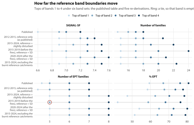
One of those band sets is degenerate, and it is worth stopping on because it is a defect in the generator rather than in the data. The 2015–2019 EPT-family boundaries come out at 5, 5, 6, 8: the top of band 1 and the top of band 2 are the same number, so band 2 is the interval \((5, 5]\), no sample can occupy it, and the factor scores 0, 1, 3, 4 or 5 but never 2. It is the ringed row of Figure 14.1, and the only row there with three points rather than four. Two of the four factors are integer-valued — the family count and the EPT-family count — so ties of this kind are routine whenever the calibration set is small, which is exactly when the reference set has been thinned by exclusions. The band generator used in this chapter now checks every column it produces and records the ties; across the five re-derived sets above — the published table is not generated, so the check cannot reach it — it flags exactly one, the EPT-family column of the 2015–2019 window (n_ept_families (5, 5, 6, 8)). An assertion that the four boundaries are strictly increasing is part of R9, and it belongs in Test 6 of the protocol as well. Where the assertion fails, the right responses are to widen the calibration window until the boundaries separate, or to collapse the tied scores into one band and say so in the published table. Silently publishing a five-point scale that cannot return one of its values is not among them.

14.3.3 The published bands already contain a fire

Table 14.2: Monitoring catchments with at least 20% of their area burnt in the 2013-14 season. The Fire(s) column carries NSW RFS incident names rather than colloquial ones: “Linksview Road, Springwood” and “Mount York Road” between them name 15 of the 18 catchments listed.

Site	Waterway	Tier	% burnt	Fire(s)
L14	Frasers Creek Tributary	Urban	100	Linksview Road, Springwood
05.2GMVR	Asgard Brook	Reference	100	Mount York Road
05GMVR	Asgard Brook	Reference	100	Mount York Road
44NYK	Frasers Creek tributary	Urban	100	Linksview Road, Springwood
W14	Bennett Gully	Reference	100	Mount York Road
42NWLR	Shaws Creek	Urban	99	Hawkesbury Road; Linksview Road, Spri…
60GBLR	Pierces Pass Creek	Reference	99	Mount York Road; State Mine
02GBLR	Jungaburra Brook	Reference	98	Mount York Road; State Mine
28EHZR	Ingar Dam	Reference	97	Mount Bedford
28.2EHZR	Ingar Creek	Reference	95	Mount Bedford
40NSV	Long Angle Creek	Urban	85	Linksview Road, Springwood
43.2NYK	Frasers Creek	Urban	84	Hawkesbury Road; Linksview Road, Spri…
04GMV	Grose River tributary	Slightly disturbed	80	Mount York Road
03BMV	Fairy Dell Creek	Slightly disturbed	60	Mount York Road
41NWL	Blue Gum Swamp Creek	Urban	48	Linksview Road, Springwood
43NYK	Frasers Creek	Urban	46	Linksview Road, Springwood
39NSV	Fitzgerald Creek	Urban	38	Linksview Road, Springwood
81NFB	Sassafrass Creek	Slightly disturbed	25	Sassafras Ridge

The 2013–14 season burnt 28 monitoring catchments, including 7 reference catchments, 4 of which supply samples to the published calibration window. That window is 2012–2015 and the fires ran from 17 October 2013, so the percentiles that define Excellent were drawn from a reference set that had already burnt.

The size of it matters, because it changes what the reset is being compared against. The published reference column rests on 43 samples from 9 sites. 21 of those 43 come from the 4 catchments that burnt over 90% of their area in 2013–14, and 11 were taken after the fires — about 26% of the benchmark.

Two things follow, and they pull in opposite directions.

• The incumbent bands are not a pre-fire benchmark, so “resetting them bakes a fire in” is not the right objection. Whatever the 2019–20 fires do to a new calibration set, the thing being replaced has a fire in it too, and nobody decided that — it is an accident of when the window was drawn.
• It is undocumented, and that is the actual defect. Nothing in the methods document records the window’s fire exposure, so a reader cannot tell that the standard Excellent is measured against was set partly by burnt reference creeks recovering. That is the argument for R4b: record the window, the site list and the burn extent of each calibration catchment alongside the band table, so the next person does not have to reconstruct this.

Section 14.4.1.1 measures what the equivalent exposure costs in the proposed ten-year window. This section is the reason that measurement is not a comparison against a clean baseline.

14.4 Fire and the reference sites

Chapter 4 established that 9 of the 15 delineated reference catchments burnt over 90% of their area in the 2019–20 fire season. Reference sites are the benchmark the whole rating system is calibrated against, so whether their communities changed is not an academic question: if the benchmark moved, every reference-relative score computed since 2020 is measured against a different standard.

A compositional shift is what the fire literature predicts, and it predicts it as a displacement followed by recovery rather than as a permanent loss: Verkaik et al. (2013) describe post-fire assemblages moving away from their pre-fire composition, driven by the ash and sediment the first post-fire storms deliver — for 1–4 years in mediterranean-climate streams, but often for 5–10 years in temperate ones, which is what these are — and Robson et al. (2018) found headwater assemblages back to indistinguishable from unburnt controls within two years — in five burnt and five unburnt Grampians reaches around the 2006 fire, during a long drought. The test below is therefore a test of displacement, and the trajectory afterwards is the thing worth watching.

The test compares each reference creek with its own pre-fire community. For every reference creek an average pre-fire community is computed from its 2014–2019 samples, and every sample from that creek is then scored by how far it sits from that average. If the fires changed the assemblages, burnt creeks should move further from their own pre-fire state after 2019 than unburnt ones did.

Table 14.3: Movement away from each reference creek’s own pre-fire community. A larger number means the community in that period looked less like the same creek’s 2014-2019 average. These are UNADJUSTED cell means. The difference and the ratio quoted below are the fitted difference-in-differences from a model carrying site, year and site-by-period terms, so they will not reproduce by subtracting these four numbers — see the box.

Creeks	Period	Samples	Mean distance from own pre-fire community
Not burnt	2014–2019	21	0.281
Not burnt	2020–2024	9	0.424
Burnt >90% in 2019–20	2014–2019	56	0.315
Burnt >90% in 2019–20	2020–2024	16	0.564

Burnt reference catchments did shift. Whether they shifted more than the background is not a question nine creeks can answer. Burnt reference creeks moved 0.12 further from their own pre-fire community than unburnt reference creeks did over the same period — about 1.9 times as far. Both figures are fitted, not read off Table 14.3: they come from the difference-in-differences term of a model carrying site, year and site-by-period effects, while the four cell means in that table are unadjusted — differencing those gives 0.106, which is the same story on a slightly smaller number. The 95% confidence interval on that difference runs -0.02 to 0.26 on the 0–1 Bray–Curtis scale and covers zero (p = 0.157, on 4.8 denominator degrees of freedom). An exact permutation of burnt status over all 84 ways of choosing six burnt creeks from nine agrees: p = 0.274.

What this record does support, and it is not nothing: both groups of reference creeks moved away from their own pre-fire communities after 2019, the burnt group moved further, and the direction is the one the fire literature predicts. What it cannot support is that the difference between the two groups is the fire rather than ordinary between-creek drift. The difference-in-differences is a difference of creek-level changes, so the yardstick it has to be measured against is how much creeks differ in their change — and on nine creeks that yardstick is longer than the effect.

What the limitation costs, plainly. This section cannot be used to say the fires moved the reference communities, and no reanalysis of these data will make it able to. There are 9 reference creeks with enough pre-fire data, of which 6 burnt, leaving 3 unburnt creeks and only 9 post-fire samples as the control. Separating a fire effect from between-creek drift would need roughly twice as many unburnt reference creeks sampled at the same intensity — which, given that only 15 reference catchments are delineated and 9 of them burnt, is not obtainable retrospectively. It is obtainable prospectively, by keeping the burnt reference catchments on the sampling calendar, which is what M14 asks for.

Figure 14.2: Reference creeks moving away from their own pre-fire communities, burnt and unburnt drawn separately. Each point is one sample, positioned by how different that year’s community was from the same creek’s 2014-2019 average; the two lines join the annual mean within each group. Colour is burn status — six of the nine reference creeks with enough pre-fire data burnt more than 90% of their catchment in 2019-20, and three did not. The vertical line marks the 2019-20 fire season. Both groups move away from their own pre-fire communities after it and the burnt group moves further, but on nine creeks that difference is not distinguishable from ordinary between-creek drift — read the two lines with the interval in the blockquote above, not as a picture of a fire effect.

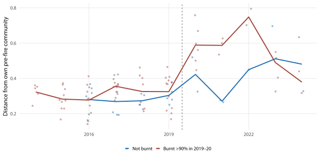
The burnt creeks’ trajectory since 2020 is consistent with recovery — the distance falls back over the following years — but with 16 post-fire samples across 6 creeks, and only a handful in the most recent years, that reading is an impression rather than a result. Chapter 13 should treat the post-2020 reference condition as provisional. That recommendation is strengthened, not weakened, by the test above coming back inconclusive: an interval running -0.02 to 0.26 is consistent with the benchmark having moved a long way as well as with its not having moved at all, and provisionality is the right treatment of a benchmark nobody can yet certify either way.

Effort sensitivity of this section. None. The distances are between relative abundances, and each creek is compared only with itself.

14.4.1 Did the fires lower the reference benchmark?

Chapter 4 established that 9 of the 15 delineated reference catchments burnt over 90% of their area in 2019–20, and that 7 burnt almost entirely in 2013–14 — inside the original band calibration window. Chapters 5 and 8 both flagged this as a threat to any re-derivation: if the reference sites are themselves degraded, bands drawn from them describe a lowered standard.

Table 14.4: Reference-comparison boundaries derived before and after the 2019-20 fires. 152 and 134 calibration samples respectively. The before-window EPT-family column is the degenerate set described above and its direction call rests on a tie.

Factor	Before (2015-2019)	After (2020-2024)	Direction
SIGNAL-SF	6.8, 7, 7.3, 7.5	7, 7.2, 7.4, 7.6	More demanding
Number of families	15, 17, 20, 24	15, 17, 19, 21	Less demanding
Number of EPT families	5, 5, 6, 8	5, 6, 7, 8	More demanding
% EPT	42.1, 58.8, 68.2, 76.4	53.9, 64.7, 72.6, 80.1	More demanding

Bands pooled from reference and slightly disturbed sites after the fires are more demanding, not less, on the sensitivity and EPT factors. That is not evidence that the fires left the benchmark alone. It does not follow, for a reason that is easy to miss: the two calibration windows do not hold the same creeks.

Table 14.5: Composition of the two calibration windows. They are not the same creeks, and the difference runs in the direction that would hide a fire effect.

Window	Calibration samples	Share slightly disturbed	Share from catchments that burnt over 90% in 2019-20
2015-2019 (before)	152	53%	37%
2020-2024 (after)	134	81%	16%

The pre-fire window is 37% samples from catchments that later burnt over 90% of their area (Table 14.5); the post-fire window is 16%. The pre-fire window is 53% slightly disturbed and the post-fire window 81%. A pooled benchmark that does not fall because the burnt creeks largely dropped out of the sample, and because the unburnt ones rose enough to carry the rest, says nothing about what the fire did.

The direct test is available: the same creeks, before against after, burnt against unburnt.

Table 14.6: Difference-in-differences on each factor, standardised: the change at burnt reference and slightly disturbed sites across the fire, relative to the change at unburnt ones. Site, year and site-by-period random effects, 286 samples at 30 sites.

Factor	Change at burnt sites, SD
SIGNAL-SF	-0.74 (-1.39 to -0.09)
Number of families	+0.41 (-0.34 to +1.15)
Number of EPT families	-0.04 (-0.66 to +0.59)
% EPT	-1.05 (-1.96 to -0.14)

Burnt reference and slightly disturbed sites lost 0.47 points of published score relative to unburnt ones across the fire (95% CI 0.04 to 0.90). The pooled comparison reads “more demanding” on three of the four factors — SIGNAL-SF, Number of EPT families, and % EPT — and two of them, SIGNAL-SF and % EPT, are the two that fall hardest once the comparison is made within site. The remaining one, the EPT-family count, is the direction call that rests on the tie in Table 14.4’s caption.

Split by factor, the within-site fall is carried by SIGNAL-SF and % EPT — the rows of Table 14.6 whose intervals exclude zero. The intervals on the family count and the EPT-family count cover zero, so those rows will not carry a claim in either direction, and the loss on the composite score rests on two of the four factors rather than on all of them.

How much does that depend on how the comparison is set up? Dropping the year term gives 0.54 points; keeping only the sites sampled on both sides of the fire — 273 samples at 28 sites — gives 0.52. Measuring burn extent from each sample’s own three-year fire history rather than from the 2019–20 season alone gives a smaller loss, 0.38, on an interval that reaches just past zero (-0.13 to 0.89): same direction, less confidence. Where the two periods are cut is not a free choice, though. The fires burnt across the 2019–20 summer and every 2020 sample at a burnt site comes after they started, so counting 2020 as “before” puts the most affected samples on the wrong side of the line, and the estimate collapses (0.07, -0.41 to 0.55). That is the cut being wrong, not the result being fragile — but the half-point figure belongs to the 2019 cut and should be quoted with it.

The comparison is imprecise, because only 5 burnt reference or slightly disturbed sites have samples on both sides of the fire — but it is the right comparison and it points the opposite way to the pooled one.

One more caution attaches to the within-site comparison, and it is about how many tests this section runs rather than about any one of them. The half-point loss is the headline of ten related tests on a single fire event — this estimate, the four factor-level differences beneath it, the four sensitivity refits above, and the compositional test of Section 14.4 — and none of them carries a multiplicity correction. The composite interval clears zero narrowly, at 0.90 on its nearer end, and an interval adjusted for a family of ten would cover zero. Correcting is not the right remedy here: ten tests of one fire are not the independent family a correction procedure assumes, and nothing in this section is chosen for being significant. Stating the family is the remedy. The half-point figure should be read as one result among ten that point the same way, rather than as a single test that cleared a threshold — and the reset recommendation of Section 14.4.1.1 rests on the class movements, which are counts rather than tests.

The 2019–20 fires did lower the macroinvertebrate benchmark at the catchments that burnt, by about half a score point. A depression of that size, at catchments burnt over most of their area, is consistent with the post-fire literature (Verkaik et al. 2013; Gomez Isaza et al. 2022), which expects it to be temporary — but not necessarily brief, and the two sources disagree about how brief. Verkaik et al. (2013)’s often-quoted “one to a few years” is their mediterranean figure; for temperate streams, which these are, the same paper reports displacement often lasting 5–10 years and recovery times running from years to decades. Against that, Robson et al. (2018) found headwater assemblages back to indistinguishable from unburnt controls within two years — in a study of five burnt and five unburnt Grampians reaches around the 2006 fire, during a long drought. That is the argument for a rolling calibration window rather than for excluding the burnt catchments permanently. The paper carries its own caution and the recommendation should carry it too: fire frequency is rising, and repeated fire may permanently alter the riparian vegetation that headwater streams depend on for shade, wood and leaf litter. A rolling window absorbs a benchmark that returns; it does not absorb one that does not. If the burnt reference catchments have not recovered within about five years, the window is the wrong instrument and the benchmark itself has to be re-derived.

Two further cautions attach to the pooled comparison, and they still hold.

• It is confounded by weather as well as by composition. The 2015–2019 window contains the 2018–19 drought and the 2020–2024 window the wet La Niña years, so part of the apparent post-fire improvement is rainfall. This is the same confound chapter 8’s fire analysis ran into, and it is what the year term in the model above is there to absorb.
• Absence of a shift in four coarse metrics is not absence of a shift. Section 14.4 finds burnt reference creeks displaced from their own pre-fire communities by about 1.9 times the background amount — though on nine creeks that difference is not separable from between-creek drift (p = 0.274), so it is a reason not to read the four metrics as the last word rather than a competing result.

14.4.1.1 What this does to the reset recommendation

The consequence needs stating carefully, because the obvious inference is the wrong one. If burnt catchments are in the calibration set and their scores have fallen, resetting the bands now would bake the fire into the benchmark and make every other creek look better by comparison — a network-wide improvement arriving through the back door. That is a real mechanism and it is worth measuring rather than asserting.

Table 14.7: What the burnt-catchment question is worth, in published ratings. The urban column is held at 2015-2024 throughout, so every difference here is the reference column.

Calibration set for the reference column	n	Top of reference % EPT band 1	Mean sample score	Samples rated differently from the recommended set
Ten-year window, burnt catchments kept (recommended)	286	47.4	2.52	0.0%
Ten-year window, burnt catchments excluded	219	51.4	2.49	2.7%
Five-year post-fire window, burnt catchments kept	134	53.9	2.48	4.6%
Five-year post-fire window, burnt catchments excluded	118	57.9	2.46	5.9%

The mechanism is real and it runs in the direction the argument expects, but it is small. Keeping the burnt catchments in the recommended ten-year window makes the benchmark slightly more lenient: the top of the reference % EPT band sits about four percentage points lower than it would without them, the mean sample score is 2.52 against 2.49, and 2.7% of samples and 1 site in 77 carry a better word than they otherwise would. That is the spurious improvement, measured — and at 2.7% of ratings it is smaller than the difference between any two of the calibration windows in Section 14.3.2.

Two things are holding it down, and neither is durable.

• The post-fire window under-represents the burnt creeks. They supply 16% of the recent calibration samples against 37% of the older ones, so they carry less weight in a benchmark drawn from the recent record than they did in the one being replaced. That advantage disappears as those catchments are re-sampled.
• The wet years pushed the other way. Across the fire the unburnt calibration sites rose 0.15 points while the burnt ones fell 0.32, so a post-fire benchmark is not depressed overall even though its burnt component is. This is why calibrating on the post-fire five years alone — the version that would most fully bake the fire in — gives a more demanding benchmark than the ten-year window rather than a more lenient one. A run of wet years is a coincidence, not a policy.

The honest summary is that the reset is safe to make now, that it is safe partly by luck, and that the check which establishes this is one line of code and should be run every time the bands are refreshed.

Recommendation R4 — what to anchor to. Reset the percentile anchors on a rolling ten-year window of reference and slightly disturbed sites, refreshed every five years, keeping the burnt catchments but publishing the excluded set beside them. Three things support that, and one of them is new. 6 of the 9 reference sites that actually enter the ten-year calibration window burnt, so excluding them leaves 3 and a calibration set too small to be stable. A fixed historical window will drift further from the network every year it is left in place. And the measured cost of keeping them, on a ten-year window, is 2.7% of ratings in the direction of leniency — small, and smaller than the difference between any two of the windows in Section 14.3.2.

Three conditions attach. First, the ten-year window is doing real work here and the recommendation should not be quietly shortened: calibrating on the post-fire five years alone changes 4.6% of published ratings relative to the ten-year window, purely by covering a different climate period. Second, publish the burnt-catchment-excluded band set alongside every reset, as Table 14.7 does. It is one line of code, it takes no judgement, and it makes the size of the fire’s influence on the benchmark visible every time the bands are refreshed instead of arguable. Third, record the window, the site list and the burn extent of each calibration catchment with the band table, so that any published rating can be traced to the benchmark it was scored against and the next reset can be checked against this one. That last one is the condition worth insisting on, and it is where we would put the effort: whoever publishes the reset should be able to say plainly that the benchmark is measurably depressed at the creeks that burnt, and that the reason this barely shows up in the bands is a run of wet years and a recent sample that happens to under-represent those creeks.

14.4.2 What resetting the bands would do to the published ratings

Table 14.8: Effect of resetting the percentile bands on bands re-derived from 286 calibration samples — reference and slightly disturbed sites, 2015-2024 — and applied to the 684 samples from 2015 onwards. The two counts are different sets: the first calibrates the bands, the second is scored against them. Samples from before 2015 are excluded, because scoring them against 2015-2024 percentiles judges the 1990s against a modern benchmark.

What is reset	Mean score	Samples changing class	Share rated Excellent
Nothing (published bands)	3.16	-	22%
Urban column only	2.97	16%	19%
Reference column only	2.99	15%	15%
Both columns	2.81	33%	13%

Resetting the bands is not cosmetic. On 2015–2024 site means, 27 of 77 sites (35%) drop exactly one rating class, 0 drop two, and 0 rise. The share of 2015–2024 samples rated Excellent falls from 22% to 13%.

The two columns contribute about equally, and they do it in different parts of the scale. Resetting only the reference column moves 15% of samples; resetting only the urban column moves 16% (Table 14.8). Where they part company is not how many samples move but which ones: the share rated Excellent falls from 22% to 19% on the urban reset alone and to 15% on the reference reset alone, so it is the reference column that takes the top of the scale away. The urban reset is the leniency of Section 13.3.1 being corrected, and it does that job in the middle of the scale.

Table 14.9: Where the reset helps and where it does not. The urban row is the share of samples scoring 4 or 5; the reference rows are the share scoring exactly 1. Over the whole 1,503-sample analysis set, 1998–2024, which is a wider population than the 684-sample 2015-onwards set of Table 14.8 above.

Column	Share at the extreme band, published	Share at the extreme band, after the reset
Urban SIGNAL-SF	76%	46%
Reference % EPT	62%	47%
Reference Number of EPT families	57%	72%
Reference Number of families	43%	50%

The reset does what it is meant to do to the urban column and the opposite to two of the reference ones (Table 14.9), and Section 13.5.7’s diagnosis needs correcting to match. Urban SIGNAL-SF is the column drawn from a distribution it is then applied to, and there the pile-up at 4 and 5 genuinely is the leniency of Section 13.3.1: the reset cuts it from 76% to 46%. The reference columns are different. They are drawn from reference sites and applied to a mostly urban network, so a pile-up at band 1 is the design working, not a reproducibility failure — and because the re-derived reference bands are more demanding than the published ones, the reset makes it worse. The reference EPT-family factor goes from 57% to 72% of samples scoring exactly 1.

That is only tolerable because Section 13.5.3 proposes removing the reference column as a separate score altogether. So there is an order of operations here, and it is the one condition in this chapter we would not bend on. R4 (this band reset) should not be adopted without R3 (chapter 15’s two-anchor scoring rule). Taken alone, the reset fixes the urban column and makes the reference comparison less informative than it is now — the share of samples scoring exactly 1 on reference EPT families goes from 57% to 72%. Taken together, the reference distribution stops being a separate score and becomes the upper anchor of one scale, and the pile-up has nowhere to happen. Chapter 15 states the same condition from its own side (Section 15.3.3).

Figure 14.3: Where sites sit under the published bands and under bands re-derived from 2015-2024 reference and slightly disturbed sites. Each point is a site; points below the diagonal have fallen.

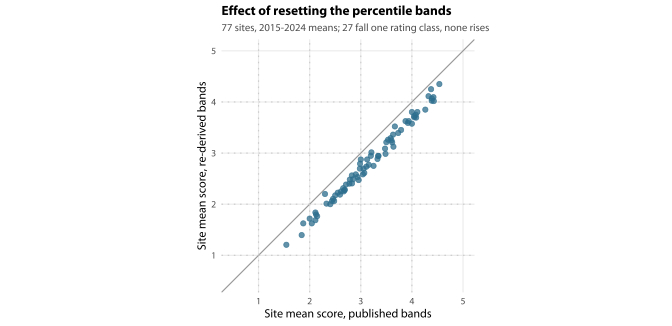
Judgement call, stated as one. Whether to reset the bands on their own is a decision about communication, not about statistics. The reset is technically correct — the published urban bands are more lenient than the distribution they claim to describe, and the reference bands were drawn from a window that closed 9 years ago. But publishing it alone would tell the public that 35% of Blue Mountains creeks got worse in a year when nothing happened to them. The suggestion in Section 19.4 is to reset the bands as part of the wider revision, publish both the old and the new rating for a transition year, and label the change explicitly as a recalibration.

14.5 What we can and cannot say

Table 14.10: What this chapter establishes, and how far each answer can be leant on.

Question	Answer	Confidence
Can the bands be reset from the reference and slightly disturbed sites?	Yes. The generator in this chapter re-derives all four boundaries from a named dataset and a named window, and the scoring function takes the new table unchanged. The recommended set is 286 calibration samples over 2015-2024.	High. This is arithmetic on data you already hold.
How much does the answer depend on which window is chosen?	Little for the boundaries, a great deal for the published words. Across the five re-derived sets in Section 14.3.2 the SIGNAL-SF boundaries move by at most 0.2 grades, but choosing the post-fire five years instead of the ten-year window changes 4.6% of published ratings.	High. All five re-derived sets are built the same way.
Do integer factors break the percentile method?	They can, and one of the five re-derived sets here shows it: the 2015-2019 EPT-family boundaries come out at 5, 5, 6, 8, so band 2 is an interval no sample can occupy and the factor can never score 2. Small calibration sets make this routine.	High. It is a property of the arithmetic, not an estimate.
Did the 2019-20 fires lower the reference benchmark?	Yes, at the catchments that burnt: 0.47 points of published score (95% CI 0.04 to 0.90) relative to unburnt sites, measured within site over 286 samples at 30 sites. The pooled before-and-after comparison says the opposite and is confounded by which creeks are in each window.	Moderate. The direction is robust to four ways of setting the comparison up, but only 5 burnt calibration sites have samples on both sides of the fire.
Did the fires change the reference communities themselves?	Not answerable on this design. Burnt reference creeks moved 0.12 further from their own pre-fire community than unburnt ones — about 1.9 times as far — but the 95% CI is -0.02 to 0.26 on the 0-1 Bray-Curtis scale and covers zero (p = 0.157; exact permutation over all 84 assignments of burnt status, p = 0.274). Both groups moved; the difference between them is not separable from between-creek drift.	Low. 9 reference creeks with enough pre-fire data, 6 of them burnt, 9 post-fire control samples. The contrast is assigned at the creek, so 9 creeks is the sample size however many samples are taken, and no adequate retrospective control exists.
Does keeping the burnt catchments in the calibration set bias the reset?	Yes, towards leniency, and it is small: 2.7% of samples and 1 site in 77 carry a better word than they would with the burnt catchments excluded. That is smaller than the gap between any two calibration windows.	Moderate. The size is measured, but two things are holding it down that will not last — the recent sample under-represents the burnt creeks, and a run of wet years pushed the unburnt ones up 0.15 points.
What does the reset do to the published ratings?	27 of 77 sites (35%) drop exactly one class on 2015-2024 means, 0 drop two, 0 rise. The share of samples rated Excellent falls from 22% to 13%.	High. Both band tables applied to the same samples by the same function.
Does the reset fix the pile-up at the ends of the scale?	For the urban column yes (76% of samples at band 4 or 5 falls to 46%); for the reference columns it makes it worse (reference EPT families, 57% to 72% scoring exactly 1). That is why the reset needs the two-anchor scoring rule with it.	High. Counted directly, both ways.
Can the currently published 2012-15 bands be reproduced?	No — chapter 13 could not regenerate them under any of six reasonable constructions. This chapter re-derives bands from a specification; it does not explain the published ones.	High that they do not reproduce. We do not know why, and that is the last of the five items on this chapter’s list above.

14.6 Three things you might want to think about

These carry the ids from Section 19.4. The prefix is not decoration: the monitoring and conservation asks are numbered from 1 as well, so a bare “recommendation 4” in an email means four different things.

1. Reset the bands on a rolling ten-year window, and not on their own — R4 with R4a. Section 14.4.1.1 has the window, the conditions, and why the order matters more than the timing.
2. Publish the burnt-excluded band set beside every reset, and record burn extent with the band table — R4b. One line of code each, no judgement needed, and Section 14.3.3 is the reason.
3. Make the generator assert that the four boundaries strictly increase — R9. One of the five re-derived band sets here fails it today.

When to publish is yours rather than ours; Section 15.4.3 is where we make the case for running both ratings for a cycle.

Gomez Isaza, Daniel F., Rebecca L. Cramp, and Craig E. Franklin. 2022. “Fire and Rain: A Systematic Review of the Impacts of Wildfire and Associated Runoff on Aquatic Fauna.” Global Change Biology 28 (8): 2578–95. https://doi.org/10.1111/gcb.16088.

Robson, B. J., E. T. Chester, T. G. Matthews, and K. Johnston. 2018. “Post-Wildfire Recovery of Invertebrate Diversity in Drought-Affected Headwater Streams.” Aquatic Sciences 80 (2): 21. https://doi.org/10.1007/s00027-018-0570-7.

Verkaik, Iraima, Maria Rieradevall, Scott D. Cooper, John M. Melack, Tom L. Dudley, and Narcís Prat. 2013. “Fire as a Disturbance in Mediterranean Climate Streams.” Hydrobiologia 719 (1): 353–82. https://doi.org/10.1007/s10750-013-1463-3.