4  Catchments, climate and fire

Blue Mountains City Council Healthy Waterways — statistical analysis

4.1 What this chapter is for

Neither database holds a single field describing the catchment upstream of a monitoring site. There is no imperviousness figure, no land use, no rainfall, no fire history — the words “DCI” and “impervious” do not appear anywhere in either file. Yet three of the questions you asked us turn entirely on catchment context:

• Any correlations with %DCI? Can we get a more accurate DCI assessment for all our monitoring sites?
• Climate links — do we have what we need? Or at least rain, drought cycles, bushfire?
• Have stormwater treatment projects, for example biofilters, achieved change?

So this chapter is the one where we built what you do not hold, out of public Australian government data, and said plainly which of those questions the result can answer. Imperviousness, rainfall and fire have nothing to do with one another as subjects. They are here together because they share one sentence: your databases hold none of this, so we built it. Whether waterway health has changed is chapter 5’s business, not ours.

Four findings here change how the rest of the report has to be read.

1. Imperviousness can be estimated for every site with a usable position, and the ranking it produces agrees with your own classification of the low-disturbance sites — but the absolute values, and the 5% line, are not reliable enough to carry a planning decision (Section 4.3.6).

2. “DCI” is retired from here on, and we say imperviousness and mean total imperviousness. Not because connection does not matter — the literature is unambiguous that it does — but because neither version of it we can build for you earns its place as a separate variable. Section 4.3.7 shows the working, including the fair test that connection was free to win and did not.

3. The reference sites burnt. 9 of the 15 reference catchments had over 90% of their area burnt in the 2019–20 Black Summer fires, and several had already burnt in 2013–14. The reference condition every “Excellent” rating is judged against is not a stable benchmark across the series (Section 4.4.3.1). And how hard a catchment burnt turns out to matter where how much of it burnt does not (Section 4.4.4.1).

4. The stormwater treatment question cannot be answered with the data as recorded — no commissioning dates in either database, no designated controls, and the Kedumba sites were established after the works. Section 17.3 sets out exactly what would fix that.

4.2 The data behind this chapter

Each question and request below is set out again in What we need from you, with what it blocks, what an answer is worth and what it would cost you to find, ranked against every other ask in the report.

4.2.1 What this chapter uses, and where it came from

Neither database holds a single catchment field — no imperviousness, no land use, no rainfall, no fire — so everything in this chapter was built from public Australian government data and from your own GIS.

Catchments are delineated from your 12 m DEM_Broadscale surface, chosen over three alternatives on a test against your own 2003 first-order catchment polygons. 129 of the 137 register sites get a catchment, giving 120 distinct catchments, because five groups hold more than one monitoring point. Imperviousness comes from NSW Spatial Services road-corridor polygons and Geocoded Addressing Theme address points, cross-checked against NSW Landuse 2017 and ABS mesh blocks. Climate is SILO daily surfaces at 34 grid cells; fire is the NPWS Fire History layer and DCCEEW’s Fire Extent and Severity Mapping.

Blocks: Nothing — this is a statement of what we used. Value: moderate. Costs you: minutes. Refer to it as dq:catchment-covariates-built-not-held.

Your AssetPipe, AssetPit and StormDischarge layers were burned into the 12 m surface and every catchment re-delineated, to find out how much of the delineation depends on pipes crossing ridges.

12,318 pipes, 259.0 km, assembled into 2,882 connected components. The answer is that the median catchment moves 0.85% and reference catchments move 0.000%, so the surface-only delineation stands — but the direction of flow had to be inferred, because the register carries no invert levels, no node ids and no direction field.

Blocks: Nothing — this is a statement of what we used. Value: moderate. Costs you: minutes. Refer to it as dq:drainage-burn-provenance.

4.2.2 What is wrong with it

Only 407 of the 2,882 connected components in the stormwater asset register reach a recorded discharge point — 20.3% of 259 km. The other 206 km stops where the register stops, not where the network stops.

The register holds no private drainage, no Transport for NSW highway drainage and no Sydney Water assets, so what is in it is a network shredded into fragments by the pieces belonging to somebody else. The median connected run is 32 m and 1,198 of the 2,882 components are a single pipe. It is not an artefact of how we snapped to outfalls: relaxing that tolerance tenfold moves the figure from 19.3% to 22.9%.

Blocks: Every conclusion in the drainage section, and the connected-imperviousness test that closed the DCI question. Value: high. Costs you: minutes. Refer to it as dq:drainage-network-truncated.

Five of the 120 catchments cross the 5% modelled DCI line, and one crosses on total imperviousness, purely from enforcing the stormwater pipes in the terrain — a defensible change of method, not a change of data.

Six crossings in all, counting the one on total imperviousness. Three sit on the line and would cross on any perturbation. Three cross for a real reason and all three are urban with a large area change. Ranks are stable to the same change (Spearman 0.98), so this is an argument about the threshold and not about the covariate.

Blocks: Any planning control expressed as a 5% cut. Value: high. Costs you: minutes. Refer to it as dq:five-percent-line-unstable.

Imperviousness charges 45% of the whole cadastral road reserve as sealed, which is an assumption applied to verge, table drain and unformed Crown road alike.

There is no attribute on the NSW cadastral layer that would separate a formed road from a paper one: classsubtype takes two values, Public and Pathway, and roadwidth is populated on 3.7% of polygons in four different units. The reserve is the entire source of any imperviousness at three of the fifteen reference catchments, and it multiplies a large area in the urban ones, so the coefficient sets the level of the reference-to-urban contrast.

Blocks: The level, though not the ranking, of every imperviousness figure. Value: high. Costs you: minutes. Refer to it as dq:road-sealed-fraction-assumed.

4.2.3 Questions only you can answer

How was the “Distance from source (m)” field measured — on what map or imagery, in what year, by whom, and along the channel or as a straight line?

It was probably meant as a descriptive field. It now steers the pour point, and therefore the whole catchment, at 90 of the 120 catchments — 94 have the field recorded, and at four of those no channel was found within reach of the length it gives, so the plain nearest-channel rule was used instead. For most of the 90 the constraint changes nothing: the median catchment moves by 0.08% against a rule that never sees the field. For 15 it moves the area outside the 0.8–1.25 band, and for 11 by more than a factor of two. The extreme is 73BKT, at 7,906 ha with the constraint against 9.5 ha without it.

Refer to it as dq:distance-from-source-provenance.

Which first_order_catchments layer should we treat as authoritative — the .shp with 1,326 polygons and non-unique IDs, or the .TAB with 526 that carries OBJECTID?

We are currently joining on name because the IDs do not support anything better, and a name join across two layers that disagree on polygon count is wrong somewhere. Every catchment-scale covariate goes through this join.

Refer to it as dq:first-order-catchments-authoritative.

How far is a typical Blue Mountains roof from the pit it drains to? We have assumed 30 m, with bounds of 15-60 m, and it is an assumption, not a measurement — your drainage engineers will know better than we do.

Median measured DCI moves from 1.5% to 4.7% across that range, and the number of catchments under the 5% boundary moves from 107 to 61 out of 120. The boundary is more sensitive to this one unmeasured distance than it is to the entire modelled-versus-measured imperviousness question we spent a chapter on.

Refer to it as dq:roof-connection-distance.

You asked for %DCI so it could go into a planning instrument, and we cannot give you a defensible numeric threshold. What do you want to do instead — and how should a band boundary apply across catchments that differ in size by a factor of thirteen thousand?

The analysis supports ranking catchments and does not support a number. On total imperviousness — the scale the ranking is built on — there is no breakpoint to find at all. The 13.05% figure you may have seen (confidence interval 6.9% to 19.2%) is on the modelled connected scale, which ranks the catchments identically and merely spaces them differently, so a threshold read off it can be a property of the transform rather than of the streams. It is too wide to legislate on even taken at face value. There is also your own banding — under 5% imp, 5-10% im, over 10% imp — and whatever replaces the trigger needs to reconcile with it or replace it explicitly.

Refer to it as dq:dci-trigger-decision.

Your own per-catchment urban connection factor runs from 0 to 0.99 with a median of 0.46. Does anyone remember what it was based on?

It is recorded as a judgement with no reasoning attached. If it was field knowledge we would like to calibrate our modelled DCI against it rather than merely rank against your labels. If nobody remembers, that is a real answer too and we will say so.

Refer to it as dq:connection-factor-basis.

Who produced the published figure of 35 urban sites under 5% DCI, and what did they run? We cannot reproduce it.

The companion figure of 13 reproduces exactly. The 35 matches no combination of connection curve and total-imperviousness bound we can construct; the nearest cell is 29. It is the same class of problem as the rating bands — a published number with no surviving working — and it is better solved by finding the file than by us guessing at it.

Refer to it as dq:dci-35-sites-derivation.

Your “Typical breakdown” sheet treats driveway and hardstand area as a fixed per-zone multiple of roof area. Was that measured anywhere, or is it a working assumption?

Either is fine; we just need to know which, because it feeds the total imperviousness estimate behind every DCI figure in the report, and as far as we can tell nobody has ever checked it.

Refer to it as dq:driveway-hardstand-ratio.

Do you want to renew the Planet / NSW Imagery Hub licence? It is funded only to the end of FY2026-27 and has no dedicated staff support now — and if it is going to lapse, we should pull what we want before it does.

There are 1,860 clear PlanetScope scenes over the study area since 2017, with two years of pre-fire baseline and 221 clear scenes through 2020. That is enough to turn fire from a yes/no covariate into a post-fire recovery trajectory, which is exactly what the depressed reference benchmark needs. This is the most time-sensitive item on the whole list.

Refer to it as dq:planet-licence-renewal.

Your own method applies 0.5 impervious to the whole formed road reserve, including unsealed Crown roads and unformed tracks. Was that intended, or is it a side effect of how the layer was built?

Cheap to answer and it matters, because reconciling our imperviousness with your own 2017-18 DCI figures is the one calibration target we have — and because we are making the same assumption at 0.45 for want of anything better. See also the ask about AssetRoadSurface, which would replace both.

Refer to it as dq:road-reserve-imperviousness.

(DCCEEW / NPWS) NPWS records a burn in 22 catchment-seasons since 2021-22 where FESM maps nothing — almost all of them prescribed. Which product should we believe?

A zero on the severity raster is not always a zero fire, and every fire covariate in the catchment, health-trend and community chapters inherits the answer. Prescribed burns are the obvious explanation — too cool or too patchy for the severity mapping to pick up — but that needs confirming rather than assuming.

Refer to it as dq:fesm-vs-npws-fires.

Do you want to buy the Nearmap AI packs and 3D/DSM coverage? You have no entitlement to either at the moment — packs.json returns 403 and there are zero 3D surveys across the LGA.

They would give ready-made canopy polygons, which would save real work. But the SEED canopy layer is the better route and it is free to a Council, so this is a convenience purchase rather than a necessary one.

Refer to it as dq:nearmap-entitlement.

(DCCEEW / NPWS) The fire layer stops naming fires before 2002, and the largest fire season in the whole monitoring record — 2001-02 — falls on the wrong side of that boundary. Is there an incident register or a season report that would name them?

This is a gap in the source rather than a defect in the layer, and it is worth saying plainly which way it runs. Of the 894 catchment-seasons the NPWS layer records a burn in, 554 carry no fire name at all — but 508 of those are before 2000, and from 2002 on every single burnt catchment-season is named. The whole of the remainder is one season: 46 of the 50 burnt catchment-seasons in 2001-02 have no name. That season is the largest in the record by area burnt across the monitored catchments, larger than 2019-20 and larger than 2013-14, so the one season a reader is most likely to ask about by name is the one the layer cannot answer for. Nothing in the report is wrong because of it: every fire covariate is built from the burn geometry and not from the name, and chapter 4’s reference-catchment table (Table 4.17) says in terms that a blank is a missing name rather than a missing row. What is lost is the ability to tie a burn in a particular catchment to a fire anyone remembers.

Refer to it as dq:npws-fire-names-before-2002.

4.2.4 What would answer them

Can we get the drainage network that is missing from the asset register — private property drainage, the Transport for NSW (formerly RMS) highway system and Sydney Water’s assets — or at least be pointed at whoever holds each of them?

Your register reaches a recorded discharge point for 20.3% of its 259 km. The rest ends at an asset boundary, so we have to put the water back on the surface there, and for most of those ends that means a street or a back yard rather than a creek. This is the single largest constraint on anything we can say about connection: we built a traced connected imperviousness and it could only be traced through a fifth of the network, which is why we can say connection did not beat total imperviousness as you can currently measure it, and cannot say anything stronger. It is also what stands between the modelled DCI you asked us for and a measured one.

Refer to it as dq:complete-drainage-network.

Could we get read access to three folders on the GIS share that currently refuse us — Data\Environment, Data\Images\Model and Data\Assets\Building?

Judging by the names, those are the likely homes of the sub-catchment polygons, the DEM rasters and your own building capture — which is to say several other items on this list. One permission change may close a handful of asks at once.

Refer to it as dq:gis-folder-access.

Does anything hold invert levels, or upstream and downstream node ids, for the stormwater pipes? AssetPipe has neither, and Depth is one value per pipe so it cannot give a gradient either.

Without them the network cannot be directed from its own attributes, so we inferred the direction: pipe ends within 1 m are the same junction, and every junction drains by the shortest path to its component’s outlet, with the 12 m surface breaking ties. Those are choices, and either of these fields would remove them outright. If they live in a maintenance or design system rather than in GIS, that is just as good.

Refer to it as dq:assetpipe-invert-levels.

Is roads/AssetRoadSurface.TAB complete enough to use as the sealed road area outright — and does it cover state roads, or only the ones you maintain?

It holds 3,564 surfaced segments with a recorded width and area, about 457 ha of measured seal at a median width of 6.0 m. That is a measurement where we currently have an assumption applied to the whole road reserve, and swapping it in is the single change most likely to improve imperviousness. We have not made it, because it moves every imperviousness figure in the report and the gap where state roads should be would then become a hole rather than a rounding error.

Refer to it as dq:measured-road-surface-areas.

Could someone re-export urban zones 20170618.csv with the computed fields actually calculated? Connectedness, Connection_factor and DCI_ha all read 0 in every one of the 1,849 rows, which cannot be right — Area_impervious_ha is non-zero throughout.

Probably a save-without-recalculating. It is the only reason we cannot use your own urban DCI component, and it is one re-export.

Refer to it as dq:urban-zones-reexport.

(Sydney Water, not you) Is there a populated sewer extract? YEARLAID, DISUDATE and PLANNUM are empty for all 37,659 features in the one we have. The September 2005 trunk mains amplification REF, the reticulation network, the amplification staging dates and the Winmalee STP discharge history would all help.

This is no longer the coliform question — that break is identical at unsewered reference catchments, so the sewer is not the cause. But nothing else dates the sewer network, and catchment history is thin without it.

Refer to it as dq:sydneywater-sewer-history.

4.3 Imperviousness: total versus directly connected

4.3.1 Why the distinction matters

Total imperviousness (TI) is all the sealed surface in a catchment: every roof, road, driveway, footpath and car park, expressed as a percentage of catchment area.

Directly connected imperviousness (DCI), also called effective imperviousness (EI), is only the part of that sealed surface which drains to the stream through a pipe or a lined channel without first passing over pervious ground. A roof whose downpipe discharges to a garden is impervious but not connected. The same roof plumbed to a kerb-and-gutter that runs to a stormwater pit is both.

The distinction is not academic, and it is the best-supported single idea in the urban stream literature. The characteristic degradation of streams draining built catchments — flashier hydrology, higher nutrient and contaminant concentrations, altered channels and a macroinvertebrate assemblage stripped of its sensitive taxa — is well enough established to have a name, the urban stream syndrome (Walsh, Roy, et al. 2005). What that literature is consistent about is that connection, not sealing, is what degrades streams. Walsh, Fletcher, et al. (2005) showed that macroinvertebrate assemblages in Melbourne streams responded to effective imperviousness and not to total imperviousness once effective imperviousness was accounted for; Hatt et al. (2004) found the same for stream water quality in the same region; and Walsh and Kunapo (2009) built the flow-path mapping method that made effective imperviousness measurable at catchment scale.

How much connection it takes is contested, and the two most-cited numbers are not the same number. Booth and Jackson (1997) put the onset of readily observable degradation in Puget Sound lowland streams at about 10% effective imperviousness, while noting that sensitive water bodies degrade well below it. Walsh, Fletcher, et al. (2005), on Melbourne streams, found ecological condition declining from very low levels of effective imperviousness and reaching a floor somewhere between 1% and 14%. They agree on the direction and on the order of magnitude: the damaging range is single-digit percentages of connected imperviousness, whereas total imperviousness of 10% may mean almost nothing if the drainage is disconnected. Work in the Sydney Basin itself reports the same gradient: Davies et al. (2010) found urban streams in Sydney’s north degraded on both in-stream habitat and macroinvertebrate assemblage relative to non-urban controls.

Two consequences follow, and both are good reasons for the framework you already have. First, a total-imperviousness figure — which is what most open datasets can give you — systematically overstates the hydrological insult, and by a factor that is not constant between suburbs: an older Blue Mountains village with table drains and unkerbed streets can have the same TI as a newer kerbed subdivision and a small fraction of the DCI. Second, retrofit works such as raingardens and biofilters change DCI while leaving TI untouched. DCI is the variable that responds to management, which is exactly why your sub-catchment classification matrix (Table 5 of the June 2025 methods document) is built on DCI bands rather than TI.

Hold that thought. Everything in this section is about the concept. What follows is about the measurement, and Section 4.3.7 is where the two part company.

4.3.2 Delineating the upstream catchment of each site

Catchments were delineated from your own 12 m DEM_Broadscale surface, built from LPI contours and covering the whole local government area. Which DEM to use was tested rather than assumed. Four elevation surfaces were available and a finer one is not automatically better: high resolution resolves the kerbs, culverts and road embankments that a coarser surface smooths over, and in an urban catchment that can route flow along a gutter or trap it behind a road. 58 of your own first-order catchment polygons, delineated in 2003 from your own data and so independent of anything here, were re-delineated from each candidate surface and scored by intersection over union against your polygon. The 12 m surface reached a median 0.945, the 4 m airborne laser surface 0.872, and the 30 m Geoscience Australia DEM-H (Gallant et al. 2011) 0.510. Each fails where the physics says it should: the 30 m cell cannot resolve a 50–150 ha divide (median 0.048 in that band), and the 4 m surface falls apart below 50 ha (median 0.045), where it routes flow along kerbs and traps it behind road embankments. The same ranking holds on a second and independent test, agreement with your mapped creek network: 92.7% of modelled channel cells land within 30 m of a mapped creek at 12 m against 81.1% at 30 m. The 4 m surface also reaches only 117 of the sites. The comparison is in data-layer/external/17-dem-comparison.R, which writes its full result to data/derived/dem_comparison.rds.

Depressions were breached by least cost, D8 flow directions and flow accumulation were computed with WhiteboxTools, and each pour point was moved onto the modelled channel before its upstream area was delineated. The median pour point moved 16 m; the furthest moved 150 m.

That distance is a straight line, and it does not say which channel the pour point landed on. The catchment delineated for a site is the upslope area of its pour point, not of the recorded coordinate, so where the snap crosses a confluence the coordinate itself can end up outside the polygon drawn for it. 53 of the 129 recorded positions do lie outside their own catchment — median 12 m beyond the divide and at most 127 m, with 27 of the 53 within a single 12 m DEM cell of it. All 120 of the 120 pour points are inside the catchment delineated from them, so this is a property of where the monitoring point was recorded rather than of the routing. The snap distance cannot detect a pour point that has crossed onto a neighbouring channel, and should not be read as though it could; what settles that question is whether the pour point drains the watercourse the register names, which is the constraint described later in this chapter.

129 of the 137 register sites have a position fit for delineation, against the 85 that carry a usable stored latitude and longitude. Both databases hold an easting and a northing for every site, and that is where the extra 44 positions come from. 129 sites received a catchment, from 120 distinct catchments: 14 sites share a catchment with another, because two pairs of codes denote one location and three waterbodies carry more than one monitoring point. Any catchment-level summary must therefore deduplicate on catchment_group.

The 8 sites still without a position are 27GLNR, L13, L4, M23, P7, U13, U39, and U44. For each of them the candidate positions are far enough apart to give a materially different catchment, and averaging two plausible positions produces a third that is wrong with certainty; they are left out rather than guessed. No imperviousness figure can be produced for them.

One methodological choice worth recording. The usual recipe snaps a monitoring point to the cell of greatest flow accumulation nearby. That is wrong for this network. You deliberately pair small tributaries with the trunk streams they join, so “largest channel within 150 m” repeatedly moved a tributary site onto the main creek — at one point giving Western Creek (56NSPR, a reference site) and Glenbrook Creek (72NSP) the same 4,511 ha catchment. Sites are instead snapped to the nearest modelled channel, constrained where possible by the channel length you already record in distance_from_source_m, via Hack’s law (Hack 1957). That constraint earns its place — without it, plain nearest-channel snapping puts reference site 52NGKR onto the Glenbrook Creek trunk at 10,329 ha instead of 1,035 ha — but it has a price. Because the field is used in the snapping, agreement with it afterwards tests nothing.

And Hack’s relation is a soft constraint, not a measurement. Hack gives the coefficient as an average that “ranges between 1 and 2.5” across his own basins, so the expected area it implies is a broad indication of scale rather than a target — which is why it is used to adjudicate between snap candidates and never to validate the result. The coefficient as published is in miles per square-mile to the 0.6, and it is applied here in Hack’s own units, converted once to 1.2729 km per km²^0.6. Applying the published 1.4 directly in kilometres would bias every expected area low by 14.7%, and because the constraint sits inside the snapping objective that bias would decide which channel cell some pour points land on.

These are not Council’s catchment polygons. Every area in this chapter is delineated from the 12 m DEM to the monitoring point itself, which is usually some way above the outlet of whatever catchment Council has mapped around it, so the two sets of areas are not interchangeable and should not be differenced. Council’s own first-order polygons are what previous Council analyses have used and they remain the right thing to quote when continuity with that work is the point; they are not used here to grade a delineation.

So the price has to be paid out loud. A Hack’s-law residual cannot double as the validation statistic, and it cannot grade a catchment’s confidence: it is the residual of the objective the search has just minimised, so a median near 1 is guaranteed by construction rather than earned. That grades convergence, not correctness.

The confidence flag every chapter conditions on is built on two quantities that are outside the snapping objective and therefore free to disagree with it.

• delineation_sensitivity. The whole delineation was run a second time under the plain nearest-channel rule, which never sees your distance_from_source_m field, and the two areas are compared. Catchment area is the denominator of every imperviousness estimate, so this is the quantity that matters: does the answer depend on which snapping rule we used?
• candidate_spread_log10. How much choice the search had — the log range of contributing area across the channel cells inside the 150 m radius. It is a property of the terrain rather than of either rule, and a large value means a confluence, where picking the cell decides the catchment.

Nesting, containment, snap method and shared pour points still feed the grade; they are now four inputs among six rather than the only honest one.

Table 4.1: Delineation diagnostics. The table is mixed-grain and the last column says which population each row is counted over: 5 of the 12 rows are over the 129 monitoring sites and 7 are over the 120 delineated catchments. The distinction is not cosmetic — the confidence grades at the foot are out of the catchments, not the sites, and the site table carries 9 more rows than there are catchments. The strongest independent test is the sensitivity row: the same sites were re-delineated under a snapping rule that never sees the recorded channel length, and the two areas compared. Nesting — where one site sits inside another’s catchment, the containing catchment must be the larger, and always is — is one input among several.

Check	Result	Counted over
Sites with a position fit for delineation	129	sites
Sites given a catchment	129	sites
Distinct catchments	120	catchments
Median distance a site moved when snapped to the channel	16 m	sites
Maximum snap distance	150 m	sites
Sites sharing a pour point with another site	0	sites
Nesting violations (a catchment containing a larger catchment)	0	catchments
Catchments whose area agrees within 0.8-1.25x under both snapping rules	105 of 120	catchments
Median sensitivity to the snapping rule (1 = no dependence)	1.000	catchments
Catchments rated high confidence	69 of 120	catchments
Catchments rated moderate confidence	38 of 120	catchments
Catchments rated low confidence	13 of 120	catchments

The median catchment in Table 4.1 has a sensitivity of 1.000: for a typical site the constraint changes nothing at all. This is not a diffuse haze of uncertainty over everything, it is 15 specific catchments, named in site_catchment_checks.rds, and 11 of them differ by more than a factor of two. The extreme is 73BKT, where the constrained rule gives 7,906 ha and the unconstrained one 9.5 ha. Those are the catchments whose area is a statement about the distance_from_source_m field rather than about the terrain, which is why we would like to know how that field was measured — it is on the list above.

One thing that grade cannot separate, and it is worth saying plainly. The sensitivity is a disagreement between two snapping rules, and a disagreement can mean the terrain left the search a real choice — or it can mean the pour point was moved deliberately. Where the register records a site on a named creek, the pour point is constrained to a channel that actually drains that creek, and the unconstrained rule is then guaranteed to disagree. The constraint placed four catchments that way (09.2BBH, 40NSV, 61BWF, and 70ELW), and two of them — 09.2BBH and 40NSV — are graded below high on that disagreement alone. The largest gap is at 40NSV, where the constraint gives 542 ha against 1,301 ha unconstrained — and the unconstrained catchment is the one that fails to drain the creek the site is recorded on, which is why the constraint exists. A grade of anything below high there records that the area depends on which rule was used, which it does; it does not mean the adopted catchment is the doubtful one. The reverse asymmetry, on the burned surface, is declared in Section 4.3.3.

Table 4.2: Monitoring sites whose catchment is flagged as unreliable — 25 sites over 17 catchments, one row per site, so a catchment carrying several monitoring points repeats with the identical area (the repeated catchments are Glenbrook Lagoon (6 sites), Bedford Creek / Bedford Creek Tributary @ Red Gum (2 sites), Garnett Creek / Garnett Dam (2 sites), and Wentworth Falls Lake (2 sites)). These are reported rather than quietly shipped; treat their imperviousness estimates with caution.

Site	Waterway	Area (ha)	Recorded distance from source (m)	Issue
P2-M6	Bedford Creek	19.3	not recorded	area depends on the snapping rule by more than a factor of two
74EBB	Bedford Creek Tributary @ Red Gum	19.3	450	area depends on the snapping rule by more than a factor of two
W14	Bennett Gully	1.5	not recorded	snapped to hillslope maximum
L14	Frasers Creek Tributary	2.4	not recorded	snapped to hillslope maximum
88GHZ	Hazelbrook Creek tributary	36.0	337	area depends on the snapping rule by more than a factor of two
62BWF	Jamison Creek	65.8	2100	area depends on the snapping rule by more than a factor of two
19BKT	Kedumba Creek	226.2	2090	area depends on the snapping rule by more than a factor of two
73BKT	Kedumba River	7906.2	16300	area depends on the snapping rule by more than a factor of two
40NSV	Long Angle Creek	541.8	4910	area depends on the snapping rule by more than a factor of two
37NSP	Magdala Creek	31.0	550	area depends on the snapping rule by more than a factor of two
13BMG	Pulpit Hill Creek trib	103.8	1710	area depends on the snapping rule by more than a factor of two
26GWF	Water Nymphs Dell	16.4	417	area depends on the snapping rule by more than a factor of two
15GKT	Yosemite Creek	126.2	1400	area depends on the snapping rule by more than a factor of two
14GKT	Yosemite Creek tributary	67.8	1070	area depends on the snapping rule by more than a factor of two
32.2EWD	Garnett Creek	87.5	1810	on standing water: shares its waterbody’s outlet catchment
32EWD	Garnett Dam	87.5	1700	on standing water: shares its waterbody’s outlet catchment
49NGK	Glenbrook Lagoon	40.5	0	on standing water: shares its waterbody’s outlet catchment
63NGK	Glenbrook Lagoon	40.5	0	on standing water: shares its waterbody’s outlet catchment
64NGK	Glenbrook Lagoon	40.5	0	on standing water: shares its waterbody’s outlet catchment
65NGK	Glenbrook Lagoon	40.5	0	on standing water: shares its waterbody’s outlet catchment
66NGK	Glenbrook Lagoon	40.5	0	on standing water: shares its waterbody’s outlet catchment
67NGK	Glenbrook Lagoon	40.5	0	on standing water: shares its waterbody’s outlet catchment
28EHZR	Ingar Dam	123.8	1580	on standing water: shares its waterbody’s outlet catchment
24BWF	Wentworth Falls Lake	220.1	970	on standing water: shares its waterbody’s outlet catchment
922	Wentworth Falls Lake	220.1	not recorded	on standing water: shares its waterbody’s outlet catchment

The lake and lagoon rows in Table 4.2 need a word of explanation. D8 flow routing needs a downhill direction out of every cell, and a flat water surface does not supply one, so a monitoring point dropped inside a lagoon has no upslope area of its own and the algorithm routes it to whichever cell it happens to land in. What comes back is a catchment describing where the sampler stood on the shore, not what drains to the water. On Glenbrook Lagoon, where six monitoring points sit within 371 m of one another, that produced 6 different catchments of 8.4 to 131.5 ha for one small lagoon — wide enough to put it in the lowest and the highest DCI band at once.

So each waterbody is delineated once, from its outlet: the cell of greatest contributing area inside its mapped polygon, with every site on that waterbody sharing the result. 11 monitoring points on 4 waterbodies are covered by this.

Table 4.3: One catchment per waterbody, delineated from its outlet, replacing one arbitrary catchment per monitoring point. Every site on a waterbody now carries the same catchment area and the same imperviousness.

Waterbody	Sites	Waterbody (ha)	Catchment (ha)	TI (%)	Modelled DCI (%)
Garnett Creek	32.2EWD, 32EWD	0.6	87.5	5.1	1.14
Glenbrook Lagoon	49NGK, 63NGK, 64NGK, 65NGK, 66NGK, 67NGK	7.9	40.5	25.8	13.13
Ingar Dam	28EHZR	0.2	123.8	0.0	0.00
Wentworth Falls Lake	24BWF, 922	11.3	220.1	18.5	7.97

One site the register calls a wetland is not in Table 4.3. 12GMB on Adams Creek is classified UrbanWetland but no mapped waterbody polygon lies within 25 m of it, so it keeps an ordinary channel pour point and is flagged rather than forced onto a waterbody that the mapping does not show.

The 120 delineated catchments range from 1 ha to 20,283 ha (median 126 ha). The largest are Erskine Creek and the lower Glenbrook Creek sites, which drain a substantial part of the southern Blue Mountains; the smallest are headwater tributaries of a few hectares.

4.3.3 What happens when we put your stormwater pipes into the terrain

A digital elevation model routes water over the ground. In a built catchment a great deal of the water is in a pipe, and pipes cross ridges. Wherever the network crosses a topographic divide, a surface-only delineation puts the land on the wrong side of it. Your own 2003 catchment methodology says the built-up areas are mainly on the ridges, which is precisely where surface routing is most likely to be wrong, so this is the one mechanism that could have undermined every catchment number above.

So we tested it, rather than arguing about it. AssetPipe, AssetPit and StormDischarge were burned into the 12 m surface and all 120 catchments re-delineated from scratch.

For the typical catchment it changed almost nothing. The median catchment changed size by 0.81% — less than one 12 m cell around the edge of a 126 ha catchment — and the ordering of catchments by imperviousness is essentially untouched (Spearman 0.98). Ground gained on one side and lost on the other cancels in that figure. Counted instead as area changing hands, which is what Table 4.4 reports, the median is 1.85%. But 29 of 120 moved by 5% or more and 17 by 20% or more, and that tail is not noise: 10 catchments overlap their old selves by less than half.

All but one of the tail is urban (the exception is a slightly disturbed catchment), and the reference catchments do not move at all. That second half is the sentence that protects the rest of the report.

Table 4.4: How far enforcing the pipes moved each catchment, by disturbance tier. ‘% of area moved’ is the area gained plus the area lost as a share of the surface-only area. It is not the change in catchment size, whose median across all 120 catchments is 0.81%: a catchment that swaps ground on two sides scores on this column and cancels on that one. Overlap is intersection over union, so 1.000 means the enforced and surface-only polygons are the same polygon. Kruskal-Wallis across tiers chi-squared 45.3, df 2, p < 0.001.

Tier	n	Median % of area moved	Max % moved	Median overlap with the old catchment	Moving 5% or more
Reference	15	0.000	0.23	1.000	0 of 15
Slightly disturbed	22	0.877	134.33	0.991	1 of 22
Urban	83	4.185	273.46	0.959	28 of 83

Reference catchments move a median of 0.000%, a maximum of 0.23%, with an overlap of 1.000 — and not one of the 15 moves as much as 5%. The reason is not subtle: 19 of the 120 catchments contain no Council pipe at all, and they are the ones that do not move. The reference-against-urban comparison this whole report rests on is not threatened by this mechanism, because there are no pipes in the reference catchments. The error is confined to catchments that contain pipe — not one of the 19 pipe-free catchments moves as much as 5% — and within them it is a spread across all 29 of the tail rather than a bias in one direction.

Movement tracks pipe density (Spearman 0.75) slightly better than it tracks imperviousness (0.72), which is the signature you would want if the mechanism is what we say it is — and it did not have to come out that way.

4.3.3.1 The direction of flow is inferred, not recorded

This matters enough to state before any of the numbers are used.

AssetPipe carries no invert levels, no upstream or downstream node ids, and no direction field. Depth is a single value per pipe, so it cannot supply a gradient either. The network cannot be directed from its own attributes, so we inferred the direction. These are choices. They are not facts, and nothing below is stronger than they are.

• Two pipe ends are the same junction if they are within 1 m of each other. There are no node ids, so the graph has to be built from coordinates. We swept the tolerance: going from 0 to 1 m removes 649 spurious components at the cost of merging 686 nodes, which is digitising slop and is what you want removed; going from 1 m to 10 m removes only 240 more while merging 4,778 nodes, which is no longer slop. The elbow is at 1 m and it is not close.
• Each junction drains by the shortest path to its component’s outlet, taken as the node within 10 m of a StormDischarge feature, or — far more often, see below — the component’s lowest node on the 12 m surface.
• Where both ends of a pipe are the same distance from the outlet, the higher ground is upstream. This fired for 8 of 12,318 pipes, so it is stated for completeness rather than because it decides anything.

Joining pipe ends through a shared AssetPit was tested and not used: it merges a further 41 components, 1.4% of them, and we preferred one stated distance to a distance plus a second rule with its own tolerance.

One phrase to avoid, because it is wrong and it is the obvious thing to write. The pipes were not “burned 5 m into the DEM”. Along each directed path the burn elevation is the running minimum of the surface downstream, less 5 m, plus a small gradient so the profile is strictly monotone. Where a pipe runs from a ridge to a valley, its upper end is carved down to the downstream minimum — that is what makes it a continuous conduit rather than a chain of notches. 5 m is the offset. The median drop is 10.9 m and the maximum 79.5 m, over 26,440 cells.

4.3.3.2 The register stops before the network does

This is the finding of the exercise, and it is the concrete thing we would like from you.

Of 2,882 connected components carrying 259.0 km of pipe and open channel, 407 reach a recorded discharge point. That is 14.1% of components and 20.3% of the network by length. The other 2,475 components — 206.4 km, 79.7% of it — end where the asset register ends, not where the network ends (Table 4.5).

Table 4.5: Where the stormwater network stops. A component with no recorded discharge point is given an inferred outlet at its lowest node, and the water is put back on the surface there.

Measure	Value
Connected components	2,882
Pipes	12,318
Network length	259.0 km
Components reaching a recorded discharge point	407 (52.6 km)
Components with no recorded discharge point	2,475 (206.4 km)
…of those, more than 50 m from a mapped watercourse	1,984
Median length of a connected run	31.6 m
Components that are a single pipe	1,198

The register holds no private drainage, no RMS highway drainage and no Sydney Water assets, so a pipe that ends because the register ends is an artificial sink. We handle those honestly — the carve stops and flow returns to the surface — but for most of them that puts the water in a street or a back yard rather than in a creek. The inferred outlets sit a median of 129 m from the nearest mapped watercourse. That is a fair description of what a gully pit does and a poor description of what happens at the end of a trunk main.

This is not a network. It is a register of assets that happens to contain one. The median connected run is 32 m and 1,198 of 2,882 components are a single pipe, because the pieces joining them up belong to somebody else and were never recorded here. Everything in this section is therefore a conclusion about the 20.3% of the drainage network that can be followed to a discharge point.

And it is not an artefact of how tightly we snapped to the outfalls. The tolerance in use is 10 m, and sweeping it from 5 m to 50 m — a ten-fold relaxation — moves the share of the network reaching a recorded discharge point from 19.3% to 22.9%, against 20.3% at the tolerance adopted. That is the first thing a sceptical reader should ask and the answer is that it does not help.

The ask. The complete drainage network — private, RMS and Sydney Water — would turn 20.3% into something near 100%, and every conclusion in this section and in Section 4.3.7 is bounded by not having it. Invert levels or node ids on AssetPipe would remove two of the three modelling choices above outright. Both are on the list at the top of this chapter.

4.3.3.3 Do the pipes actually cross divides?

The premise of the whole exercise, tested from a completely different direction — your first-order catchment polygons tile the LGA, so a pipe whose two ends fall in different first-order catchments has crossed a mapped divide. No DEM burning is involved.

249 pipes of 12,318 (2.0%), carrying 7.6 km, cross a divide, and 168 of 2,882 components span more than one first-order catchment. So the premise is true — pipes do cross divides here — but it is true of one pipe in fifty rather than of the network as a whole, which is the first hint of why the delta above is so small.

One caveat, because it would be easy to oversell this number: those first-order catchments were themselves delineated from the same 12 m DEM. So this measures crossings of a modelled divide. That is arguably the right thing to measure, a modelled divide being exactly what a surface-only delineation gets wrong, but it is not independent ground truth and should not be quoted as one.

4.3.3.4 Where it does bite: the 5% line

Everything else about imperviousness in this report is a rank, and ranks are stable to the burn. The 5% cut is the exception, because it is an absolute threshold rather than an ordering.

Table 4.6: How many of the 120 catchments sit below the 5% line before and after the pipes are enforced, and how many change side. On modelled DCI the total moves by two catchments because the four crossings run in both directions and partly cancel; on total imperviousness the total moves by one catchment on a single crossing, so there is nothing to cancel.

Measure	Surface only	Pipes enforced	Crossing
Catchments below 5% modelled DCI	73	75	4
Catchments below 5% total imperviousness	36	37	1

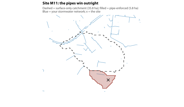
4 catchments of 120 change side on modelled DCI and 1 on total imperviousness (Table 4.6). Of the five, two — 25.2GWF on total imperviousness and 33GHZ on modelled DCI — are sitting on the line and cross on a rounding-scale move: the index shifts by 0.15 and 0.17 points on an area change under 1.8%. They would cross on any perturbation at all and their crossing says nothing about pipes. The three that cross for a real reason (M5, M11 and 26GWF, all on modelled DCI) are all urban and all have a large area change — 29% to 84% of the surface-only area, against under 1.8% for the two above.

Section 4.3.6 already argues for ranking rather than thresholding, on two grounds. This is a third and independent one: the 5% classification is not stable to a defensible change in how the water is routed, for 4 of 120 catchments — and for three of them the instability is real rather than rounding. A threshold that reclassifies 3% of catchments when you change the routing is not carrying the weight that has been put on it.

Figure 4.1: One catchment where the pipes changed the answer completely. M11’s surface-only catchment and its pipe-enforced catchment share no area at all — they meet along a boundary and nowhere else: the terrain routes this site’s drainage from 36 hectares to the north, while the stormwater network routes it from 6 hectares to the south, which is where the site itself sits. M11 is also one of the catchments that changes side on the 5% line, and it is urban.

What this exercise cannot answer. It holds the DEM fixed by construction, so it says nothing about whether the 12 m surface is the right one in the urban tail — which is exactly where the tail lives. That question needs a different test and we have not run it.

And one asymmetry we should declare rather than let you find. The pipe-enforced catchments are re-snapped and re-delineated from scratch on the burned surface, and that snap does not carry the named-creek constraint the surface delineation now uses — the rule that a pour point must actually drain the watercourse the site is recorded on.

It moves the surface pour point for four of the 120 catchments (09.2BBH, 40NSV, 61BWF and 70ELW). For two of those — 61BWF and 70ELW — the two arms still agree about most of the catchment. For two they do not: 09.2BBH and 40NSV are the sites the constraint moved onto their own creek, and their pipe-enforced catchments are still on the creek the surface delineation used to be on, so the two now share almost no area. The disagreement this comparison reports at those two sites is the constraint, not the pipes, and neither should be read as evidence about stormwater routing. Bringing the constraint into the burned delineation would remove the asymmetry; that is a change to a second delineation rule and it has not been made here.

4.3.4 Estimating total imperviousness

No open building-footprint layer is published by the New South Wales portals — a search of the NSW SEED data portal for “impervious” returns no datasets at all, and neither SEED nor the Spatial Services portals carry footprints. An open national layer does exist, though, and this project holds it: Microsoft’s GlobalMLBuildingFootprints, 239,073 AI-derived footprints over the study window, published under a permissive open licence. The two class-based estimates below still model roof area, from land-use classes and from mesh blocks. Method ST — the one this report adopts — no longer does: its premises term is roof area measured from Council’s Geoscape building polygons, plus paving at a multiple of that roof area set by the building’s planning zone. Section 4.3.7 measures roof area from the same layer, so the two halves of this chapter now treat it the same way. Until 29 August 2026 ST assumed 250 m² of roof and paving per addressed premises instead, and the paragraph below records what changed when that assumption was retired.

One thing here was unresolved for months, and this is what became of it. Both download registers describe the open footprints as replacing the 250 m² per address point that method ST assumed, and for a long time the code did not do that: the footprints reached only the traced connected estimate, ti_primary was still a modelled roof area, and this section said so. The replacement has now been made. Method ST’s premises term is measured roof area — building polygons summed inside each catchment — plus paving at a multiple of roof area set by the building’s planning zone, so nothing in this report’s imperviousness now rests on an assumed area per premises. Two qualifications belong with that. The layer is Council’s Geoscape, not the open one described here: it is the same measured layer Section 4.3.7 uses, so the two halves of this chapter treat roof area the same way, which they did not before. And the assumption turned out to have been about a tenth low, not high: measured roof and paving come to 275 m² per address point against the 250 m² assumed, and the roof alone to 202 m² — so the level barely moved, and neither did the ordering the report actually uses (Spearman 0.99 between the retired estimate and the adopted one, over every delineated catchment). What the assumption could not supply was variation between catchments, which a constant per address point cannot, and that is what the measurement adds. The scenario band moved with it and is now narrower: Section 4.5 sets out what it does and does not span.

Three independent estimates were built:

Table 4.7: The three independent estimates of total imperviousness.

Method	Built from	Main assumption
ST — structural	Cadastral road-corridor polygons (NSW Spatial Services) and Council’s Geoscape building footprints, both measured inside each individual catchment.	45% of a road corridor is sealed carriageway plus footpath; paving per building is a multiple of its measured roof area, set by its planning zone (0.40 in the residential zones that dominate this LGA). Roof area itself is measured, not assumed.
LU — land use	NSW Landuse 2017 v1.5 (SEED), ALUM classes intersected with each catchment.	Published impervious fractions per land-use class (0.50 urban residential, 0.85 commercial, 0.80 industrial, 0.02 agriculture, 0.00 conservation).
MB — mesh block	ABS 2021 mesh block boundaries and land-use category.	Published impervious fractions per mesh block category.

Figure 4.2: The three total-imperviousness estimates compared. The land-use estimate ranks catchments much as the structural one does and the mesh-block estimate less closely, and both sit at different levels: the class-based estimates (land use and mesh block) are systematically higher than the structural estimate, because their impervious fractions are calibrated on metropolitan suburbs and Blue Mountains development is large-lot and heavily treed.

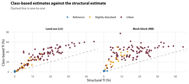
The land-use estimate orders the catchments much as the structural one does — Spearman’s rho is 0.93 between them — but the mesh block estimate agrees less well, at 0.73, which is a moderate monotone association rather than the same ordering. All three methods rank the catchments broadly alike; the mesh block estimate least so. The levels differ substantially, and that disagreement is itself the finding: the land-use estimate runs about 2.1 times the structural estimate and the mesh block estimate about 3.0 times. Both are medians of per-catchment ratios whose denominator is floored at 0.5% imperviousness, which binds for 14 of the 120 catchments — 11 of them structurally zero, where the ratio has no value to take. Dropping the floor and those zeros moves the two medians to 2.1 and 2.7, so the floor is not where the disagreement comes from.

The reason is that both class-based methods assign a fixed impervious fraction to a whole polygon of a given class, and those fractions come from metropolitan studies. A “residential” mesh block in Blackheath is not the same thing as a residential mesh block in Parramatta: lots are large, canopy is dense and much of the block is not sealed at all. The clearest symptom is that the mesh block method cannot return anything close to zero for a national park, because ABS categorises those blocks as “Parkland” rather than as wilderness.

The structural estimate is therefore adopted as the headline figure. Both of its inputs — the surveyed area of road corridor, and the roof area of the buildings — are measured inside each individual catchment, rather than inferred from a fraction assumed for a whole class of land. That is a real advantage over the class-based methods, and it is the reason for the choice.

It is only half the story, though. What turns those measurements into an impervious area is still assumed — 45% of a road corridor sealed, and paving at a multiple of roof area — exactly as the class fractions are, and the road coefficient is doing more work than it looks. road_corridor_ha is the whole cadastral road reserve, not a carriageway, and the reserve includes verge, table drain and, in this LGA, a great deal of unformed Crown road through bushland. At 2 of the 15 reference catchments that reserve is the only source of any modelled imperviousness at all, because they contain no buildings whatsoever (Section 4.3.6).

We looked for an attribute that would separate a formed road from a paper one and there isn’t one: classsubtype on the NSW cadastral layer takes two values, Public and Pathway, and roadwidth is populated on 3.7% of polygons in four different units. But you have measured this yourselves. roads/AssetRoadSurface.TAB holds 3,564 surfaced road segments with a recorded width and area — 457 ha of measured seal, median width 6.0 m. That layer would retire the 45% assumption outright rather than bounding it, and it is the single change most likely to improve these numbers. We have not made it, because it moves every imperviousness figure in the report and that is a decision for you rather than a fix for us — it is on the list at the top of this chapter.

The two coefficients are carried through as a scenario range on every reported figure; what that range does and does not cover is set out below.

4.3.5 From TI to DCI: a modelled conversion, not a measurement

True DCI requires knowing which impervious surfaces drain to a pipe, and that means your stormwater drainage network — pipe and pit layers, kerb and gutter, property drainage connections. Those layers are council-held and are not in any open dataset. No connection model has been fabricated here.

Instead DCI is converted from TI using Sutherland’s empirical relations between total and effective impervious area (Sutherland 2000), which are the standard tool where drainage data are absent. Sutherland names five basin classes; three of them are used here, under his own labels. All quantities are percentages of catchment area:

• average basins — typical suburban drainage: \(\mathrm{DCI} = 0.10 \times \mathrm{TI}^{1.5}\)
• somewhat disconnected basins: \(\mathrm{DCI} = 0.04 \times \mathrm{TI}^{1.7}\)
• highly connected basins: \(\mathrm{DCI} = 0.40 \times \mathrm{TI}^{1.2}\)

Each is stated in the source for \(\mathrm{TI} \ge 1\)%, and the family was calibrated on basins with \(\mathrm{TI} \ge 4\)%. Below 1% the figures here are an extrapolation outside the relation’s stated domain, and below 4% outside its calibration set; the effect is small in absolute terms — the central equation returns 0.035% DCI at \(\mathrm{TI} = 0.5\)% — but it is why reference catchments should be read as “at or near zero” rather than as a modelled value.

The first is used as the central estimate. The other two, applied to the low and high ends of the structural TI band, give the reported bounds — so dci_lo is a plausible low, not a floor. Sutherland’s bottom class, extremely disconnected (\(\mathrm{DCI} = 0.01 \times \mathrm{TI}^{2.0}\)), is not used: at \(\mathrm{TI} = 20\)% it returns 4.0% where the bound used here returns 6.7%, so the scenario range stops short of what his family allows at the disconnected end. Every DCI figure in this report is therefore modelled, and should be written as such wherever it is published.

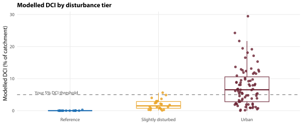
dci_lo and dci_hi are a scenario range, not a confidence interval. They vary exactly three things: the road sealed fraction (35–55%), the paving allowance per unit of roof area (halved and doubled, which brackets the residential zones of this LGA exactly) and Sutherland’s connection class. The roof area itself is measured and carries no band at all, which is why this range is narrower than the one it replaced. They carry no coverage probability, and — more importantly — they do not span the disagreement between the three imperviousness methods documented above. DCI computed from the land-use estimate falls inside [dci_lo, dci_hi] for only 35 of the 120 catchments, and from the mesh-block estimate for 13. The real spread across defensible methods is about 1.9 times the width of the reported band. Write DCI figures as “X% (scenario range A–B on the structural estimate)”, never as “X% ±”.

Figure 4.3: Modelled directly connected imperviousness by disturbance tier, one point per delineated catchment rather than per monitoring site. The dashed line is your own 5% DCI threshold, which is part of the definition of the ‘slightly disturbed’ tier in Appendix 2 of the methods document.

Table 4.8: Total and modelled directly connected imperviousness by disturbance tier, over the 120 delineated catchments rather than the 129 monitoring sites. TI is the structural estimate.

Tier	Catchments	Median TI (%)	Median DCI (%)	Max DCI (%)	Under 5% DCI
Reference	15	0.0	0.00	0.3	15 of 15
Slightly disturbed	22	6.1	1.50	5.6	21 of 22
Urban	83	16.2	6.52	29.5	32 of 83

4.3.6 A consistency check against your own tiers

Appendix 2 of the methods document names 22 urban sites as ‘slightly disturbed’, a tier defined as having less than 5% DCI together with less than 5% active agricultural land and consistently good to excellent macroinvertebrate health. Those 22 sites, plus the reference sites, are the only external information about DCI we have.

Be precise about what a comparison against them can and cannot establish. The methods document never records how the DCI figure behind the ‘slightly disturbed’ label was obtained, so this is a comparison of a model against a label of unknown numeric provenance. It can show that the two are consistent. It cannot measure accuracy, and it is not a validation of the DCI model. This section reports it as the consistency check it is.

Table 4.9: Modelled DCI against the tiers assigned in methods Appendix 2. That definition places reference and ‘slightly disturbed’ sites below 5% DCI.

Modelled DCI	reference / slightly disturbed	urban
DCI <5% (predicted)	36	33
DCI >=5% (predicted)	1	59

The reference half of the comparison is guaranteed, not tested. All 15 reference catchments come out below 0.26% DCI. 10 of the 15 contain neither a building nor a cadastral road corridor, so their structural imperviousness is exactly zero by arithmetic; 12 hold no building at all and 14 no addressed premises. The 4 that do hold road reserve carry 1.1–11.5 ha of it, to which the model applies a flat 45% sealed fraction, and that reserve is very nearly the whole source of their non-zero figure. Between them the 15 reference catchments hold eighteen buildings. Since ti_st is built from measured roof area and road corridor, and these catchments have almost neither, no estimator of any kind could have returned much other than zero here. This half of the comparison confirms that the inputs are absent. It is not a result the model could have failed.

The informative comparison is ‘slightly disturbed’ against ‘urban’. 21 of the 22 ‘slightly disturbed’ sites are placed below 5% DCI (Table 4.8), as the definition requires. The single exception is 22.2BWF (Lillians Glen) at 5.6% DCI — one site a little over the line. But 33 of the 92 urban sites also fall below 5% (Table 4.9), which is 36% of the urban tier. Some of those will be genuinely low-DCI catchments that fail the tier on health or agricultural-land grounds rather than on imperviousness, because the ‘slightly disturbed’ definition requires all three. But two in five of the urban tier is too many for that to be the whole story. A threshold that 95% of ‘slightly disturbed’ sites pass and 36% of urban sites also pass is sensitive but not specific, and the honest reading is that 5% modelled DCI does not cleanly separate the two classes.

Figure 4.4 puts that in one picture, sweeping every possible threshold rather than just 5%. The number printed beside each panel is the area under the ROC curve, or AUC, and because it is the first one in this report it is worth saying in words what it is. Take one catchment Council calls reference or ‘slightly disturbed’ and one it calls urban, at random: the AUC is the chance that modelled DCI puts the little-disturbed one lower of the two. 0.5 is a coin toss, because the score is then telling you nothing about which is which, and 1.0 is perfect separation, where the most impervious low-disturbance catchment still sits below the least impervious urban one. It reads directly as a percentage of pairs got the right way round. Chapter 13 uses the same statistic on the rating score itself (Section 13.4).

Figure 4.4: How well modelled DCI reproduces your own disturbance tiers, with and without the reference catchments. One row per delineated catchment, not per monitoring site, so that a waterbody shared by several points is counted once. Each curve sweeps every possible DCI threshold; the marked point is the 5% threshold. The reference catchments cannot fail the comparison, so the right-hand curve — ‘slightly disturbed’ against urban only — is the one that carries information.

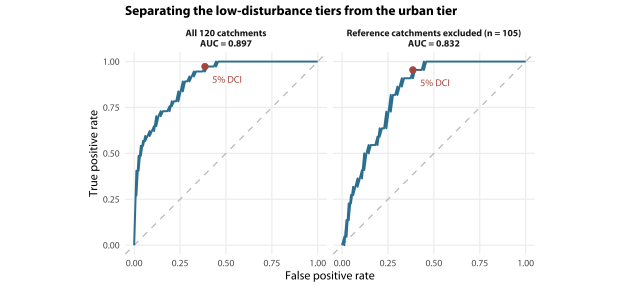
Dropping the reference catchments — the only part of the comparison that could have failed — leaves 105 catchments and an area under the ROC curve of 0.832, against 0.897 for the full set. That is a genuine and respectable result, and it is the figure that should be quoted. It says the modelled DCI orders Blue Mountains catchments in a way that broadly agrees with your own judgement of which ones are little disturbed.

Two further cautions about what that number is measuring.

It does not test the conversion from imperviousness to DCI at all. Sutherland’s relation is strictly increasing, so it cannot reorder anything: the AUC for raw structural imperviousness is 0.897, the same figure to four decimal places. The Oregon-calibrated conversion and the unkerbed-street caveat — the two uncertainties this chapter flags as dominant — cancel out of this statistic entirely, and Section 4.3.7 is what follows from that.

The discrimination is carried by one input, not by the model. Address points per hectare, a raw count with no assumed coefficient in it at all, separates the tiers at AUC 0.819 on the informative set, against 0.832 for the modelled figure built on top of it — slightly better, and the same on the full set (0.887 against 0.897). Quoted on the informative set because that is the set this section has just said should be quoted. Any later chapter tempted to describe imperviousness as the strongest catchment-scale predictor should note that on this evidence it is no better than address density.

Table 4.10: How the 5% DCI result depends on which total-imperviousness estimate is adopted. The criterion is a threshold, not a ranking, so the level of the estimate decides the answer. The medians are over the 120 delineated catchments; the three counts are over the monitoring sites Appendix 2 assigns a tier to, which is the grain of the ‘21 of 22’ result they qualify.

Method	Median TI (%)	Reference under 5% DCI	‘Slightly disturbed’ under 5% DCI	Urban under 5% DCI
Structural (ST) — adopted	11.3	15 of 15	21 of 22	33 of 92
Land use (LU)	27.7	15 of 15	10 of 22	9 of 92
Mesh block (MB)	33.6	15 of 15	4 of 22	4 of 92

And the “21 of 22” result depends on the method chosen in Table 4.7. Because the criterion is a threshold rather than a ranking, the level of the imperviousness estimate is decisive — and the structural estimate this chapter adopts is the lowest of the three. Under the land-use estimate only 10 of the 22 ‘slightly disturbed’ sites fall below 5% DCI, and under the mesh-block estimate only 4 (Table 4.10). The structural estimate is adopted for good reasons, set out above, but it is also the method most favourable to this particular claim, and that should be said.

A frank statement of accuracy. The modelled DCI is good enough to (a) rank catchments, and (b) serve as a continuous covariate in the models in later chapters. It is not good enough to be read as an absolute percentage for an individual catchment, to place a catchment confidently either side of the 5% line, or to be reported to two significant figures. It should never be described as a measurement or as validated. Roof area is no longer among the uncertainties — it is measured. The two that dominate now are the paving that goes with that roof, assumed at a multiple of roof area read off the planning zone, which sets the level in residential catchments, and the Sutherland conversion (a relation fitted to 42 subbasins around Portland and Salem, Oregon, whose off-centre variants are the author’s engineering judgement rather than fits at all, applied here to a region with an unusual amount of unkerbed street) — and, as above, neither is tested by anything in this section.

That is not an argument for caring less about imperviousness. It is the argument for using it as an ordering of catchments rather than as a number to hang a threshold on, which is what Section 4.3.3.4, judgement call 6 and judgement call 8 each arrive at from a different direction.

4.3.7 Why we stop saying “DCI” here

%DCI is the language of the question you asked us, and it is the language of your own sub-catchment framework. So this needs saying carefully rather than in passing: from here to the end of the report we write imperviousness, and we mean total imperviousness. Not because the connection idea is wrong — Section 4.3 is the case for it and we stand behind every line of it — but because neither of the two connection measurements we can build for you is a different variable from total imperviousness in any way that changes an answer.

The modelled DCI is total imperviousness with the axis relabelled. Sutherland’s relation is strictly increasing, so applying it cannot reorder anything: the Spearman correlation between dci_modelled and total imperviousness is 1.000 — one, exactly, not approximately. Under any rank statistic, any threshold expressed as a percentile, and any monotone model, they are the same variable wearing two names. That is not a criticism of Sutherland’s curve. It is what a curve fitted to total imperviousness necessarily does when there is no drainage data to feed it.

And the curve’s provenance points the same way. Sutherland’s relations come from around 42 subbasins in Portland and Salem, Oregon; only the central equation is a fit, the connected and disconnected variants being his stated engineering judgement; and every one of them is given for TI ≥ 1% and calibrated on TI ≥ 4%. That is not a criticism either — the source is honest about all three, and it remains the right tool where drainage data are absent. It is a reason not to carry the number it produces as a separate variable in a Blue Mountains report, which is precisely what we stop doing here.

And then we gave connection a fair test with a genuinely different variable, and it lost. The drainage burn made a traced connectivity possible for the first time: an impervious surface counts as connected if it drains to a pipe, and it is credited to the catchment its pipe actually discharges into, which need not be the catchment it sits in. A Sutherland curve cannot do that, because it is a function of total imperviousness and nothing else. This one is genuinely different — its Spearman correlation against total imperviousness is 0.888, not 1.000 — so it was free to win.

Table 4.11: Four ways of measuring imperviousness against median waterway health, over 118 catchments. A more negative number is a stronger association. Modelled DCI and total imperviousness agree to three decimals because they are the same ranking.

Predictor	Spearman with median health score
Total imperviousness (pipe-enforced catchments)	-0.382
Total imperviousness (surface-only)	-0.390
Modelled DCI	-0.382
Traced connected imperviousness	-0.328

Connected imperviousness is the weakest of the four (Table 4.11). The difference against total imperviousness is +0.054 (95% CI -0.037 to +0.150, 2,000 bootstrap resamples of catchments), and a positive difference means connected did worse. The interval crosses zero, so the fair statement is that connection did not beat total imperviousness rather than that it is definitely worse.

The sample-level fits say the same thing and say it four times, on 1,976 samples at 126 sites over 1998–2024, each model carrying a site and a year random effect:

Table 4.12: Total against traced connected imperviousness on four responses, same samples, same model form, one predictor swapped. Lower AIC is better; a difference inside about two points is noise.

Response	n	AIC, total imperviousness	AIC, traced connected	Difference	Connected wins?
Health score	1,976	4043	4042	-0.67	no
SIGNAL-SF	1,976	2874	2875	+1.91	no
Family richness	1,976	11206	11211	+4.81	no
%EPT	1,976	17173	17178	+4.65	no

Not one response in Table 4.12 prefers it by more than noise. One of the four — the health score — carries a lower AIC under connected imperviousness at all, and it does so by 0.67 points, inside the two the caption calls noise; on the rule the table applies, none of the four clears that bar. Connected imperviousness also explains less of that same response — marginal R² 0.093 against 0.095 for total.

The honest caveat, and it is a large one. That traced connectivity is traced through a register that reaches a recorded discharge point for 20.3% of its length, and only 19.0% of the connected building area sits on a component with a recorded outfall (Section 4.3.3.2). This is a fair test of connected imperviousness as you can currently measure it. It is not a fair test of connected imperviousness as a concept, and those are different claims. If the complete network arrives, the test is worth running again — the code is written and it takes minutes.

So the practical consequence is small, and it is not the retreat it might look like. Everything your framework does with %DCI — ranking sub-catchments, prioritising works, comparing one catchment against another — it can do with imperviousness and get the same order, because the two rankings are identical to three decimal places. What changes is that we stop reporting a number that implies we measured the connection when we did not. One variable, one name, and a scale on which we can say what was counted.

Figure 4.5: Monitoring catchments shaded by total imperviousness. The urban ribbon along the Great Western Highway shows as a chain of high-imperviousness headwater catchments. The eight catchments larger than 2,000 hectares — on the Erskine, Glenbrook, Kedumba, Cedar, Megalong and Bedford systems — are dominated by national park, and they run from 0.0 to 4.3 per cent, which on this square-root ramp is pale cream through to mid-orange rather than near zero. None of them drains to the Grose. The 45 catchments that do are the ridge-top creeks at the dark end of the ramp, every one under 400 hectares and their median imperviousness 13.2 per cent. Shading by modelled DCI instead gives an identical ordering, which is Section 4.3.7’s point.

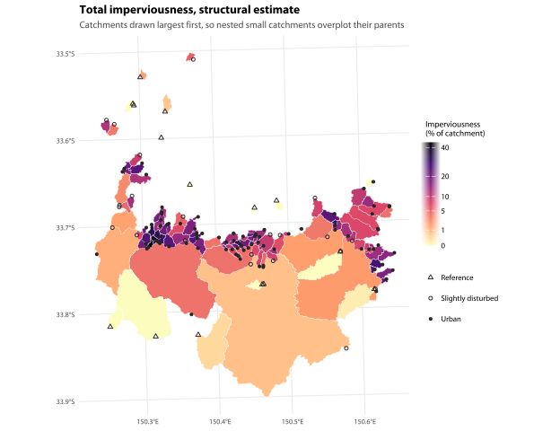
4.3.8 Filling in your sub-catchment classification matrix

Table 5 of the June 2025 methods document crosses ten-year average waterway health against three imperviousness bands to assign each sub-catchment a management approach. It could not be reproduced from the databases, because they hold no imperviousness figure. It can now be populated — and the waterbody sites go in with everything else, because they now have one defensible catchment each rather than one arbitrary catchment per monitoring point.

Table 4.13: Monitoring sites placed in your sub-catchment classification matrix, using modelled DCI and the mean health score from 2015 on. Columns are your own DCI bands. This is a site-level rendering of a matrix applied at sub-catchment level, offered as a worked demonstration that the matrix is now computable.

Waterway health (10-year average)	Under 5%	5-10%	Over 10%
Good/Excellent	36	9	1
Poor/Fair	12	9	19
Unknown health	21	14	8

Table 4.14: All 14 catchments in the ‘Active Management’ cell: over 10% modelled DCI and poor to fair health, averaged over the sites on each. These are the catchments your own framework nominates for detailed investigation and on-ground stormwater works. Imperviousness is a ranking rather than a measurement, so read this as an order of priority and not as a set of numbers.

Waterway	Sites	Catchment (ha)	Modelled DCI (%)	Health 2015-24
Kedumba Creek	86BKT	46	29.5	2.30
Leura Falls Creek	59BLA	39	24.3	2.40
Katoomba Creek	16GKT	83	19.4	2.55
Leura Falls Creek	58BLA	73	18.1	2.15
Leura Falls Creek	20BLA	215	15.3	2.78
Lapstone Creek	48NGK	130	13.6	2.00
Glenbrook Lagoon	49NGK, 63NGK, 64NGK, 65NGK, 66NGK, 67NGK	41	13.1	2.34
Lawson Creek	55ELW	43	12.9	2.68
Kedumba Creek	85BKT	125	12.6	2.12
Water Nymphs Dell	26GWF	16	12.4	2.44
Popes Glen Creek	07GBH	165	11.9	2.71
Gordon Creek	21BLA	175	11.9	2.11
Jamison Creek	62BWF	66	11.5	1.54
Springwood Creek	36GSP	219	11.5	2.50

The 11 sites on standing water are in Table 4.13, which needed a defensible figure for each of them — a D8 pour point on a flat water surface is arbitrary, so the six Glenbrook Lagoon points were carrying six different catchments and six different figures, putting one small lagoon in the lowest and the highest band at once. One caveat travels with them, and it is worth stating at its size. Nine of the 86 sites the matrix places on a health band are lentic waters, scored against the wetland band table rather than the stream one, and the matrix was built for streams. No single site’s ten-year mean mixes the two scales — every site is one or the other, and the chunk above stops the render if that ever stops being true — but a cell of the matrix can hold both, so a lentic site and a stream site sitting in the same cell got there on different rulers. Whether a lagoon belongs in a table that nominates catchments for capital works is your call rather than ours, but the figure it would be taken on now exists.

4.4 Climate, drought and fire

4.4.1 Rainfall

Daily rainfall, temperature, vapour pressure and solar radiation were extracted from SILO (Queensland Department of Environment, Science and Innovation), the Bureau of Meteorology-derived interpolated daily climate surface, from 1995 to the present. Rainfall in the Blue Mountains varies strongly with elevation — the sites with coordinates span 30 m to 978 m above sea level — so a single station would misrepresent most sites. Extractions were made at 34 SILO grid cells covering every site with coordinates, and each site is assigned its own cell. Sites without coordinates are given the regional mean and flagged, rather than dropped.

Figure 4.6: Annual rainfall over the monitoring network and the standardised precipitation index, with the major drought and wet periods marked. Any apparent trend in waterway health that follows this shape is a candidate drought signal rather than a management signal.

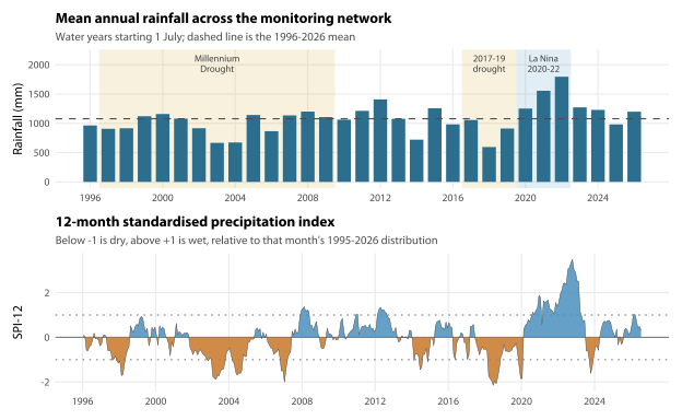
The driest water year in the series is 2018 (595 mm, 55% of the long-term mean) and the wettest is 2022 (1,795 mm, 167%). 4 water years fall below 80% of the mean and 3 exceed 125%. The monitoring record therefore spans a very large climatic range, and any comparison between the 2000s and the 2020s is partly a comparison between a dry decade and a wet one.

The drought index used throughout this report is the standardised precipitation index at 3 and 12 months, which expresses accumulated rainfall over a window as a standard normal deviate against that window’s own historical distribution (McKee et al. 1993). It is used because it is scale-free — an SPI-12 of −1.5 means the same thing at Blackheath as at Glenbrook, which a millimetre figure does not.

4.4.2 Antecedent conditions at each sample

Table 4.15: Antecedent climate covariates joined to every macroinvertebrate and water quality sample. The medians and ranges printed here are over the 2,062 macroinvertebrate samples only, not over the 2,688 water quality samples. Not every covariate is available for every sample: Days since rain over 10 mm is undefined for 73 of the macroinvertebrate samples and 33 of the water quality samples — so every cell in that row is computed over the samples that carry it, not over all of them.

Covariate	Median (range) across macroinvertebrate samples
Rain in the previous 24 hours (mm)	0.0 (0-112)
Rain in the previous 7 days (mm)	11.0 (0-301)
Rain in the previous 30 days (mm)	77 (0-786)
Rain in the previous 90 days (mm)	312 (19-1208)
Rain in the previous 365 days (mm)	1106 (375-2827)
Days since rain over 10 mm	10 (0-150)
SPI-3 at the time of sampling	-0.20 (-2.7 to 3.0)
SPI-12 at the time of sampling	0.08 (-2.5 to 3.6)

Figure 4.7: The drought or wet state in which each year’s macroinvertebrate samples were collected. Sampling through the 2000s took place under a persistently dry decade — all 6 years from 2002 to 2007 have a negative median SPI-12, though only 2 of them reach minus one — and the single driest year sampled is 2018, at a median of -1.9. Sampling in 2022 took place under the wettest conditions in the record, at a median of 2.4.

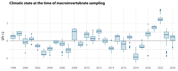
Every window in Table 4.15 ends the day before the visit. Include the sampling day and the 24-hour figure is partly rain that fell after the sample was taken, which is the one variable in the block that cannot be given a causal reading — and it is not a small effect, because it rained on the day of the visit for 2,354 of the 4,750 samples in the climate table (49.6%), or 1,344 of the 2,629 site-days those samples cover (51.1%) — the table stacks the two databases, so one visit can contribute two rows. The same-day figure is kept under its own name, rain_sampleday, because it is a perfectly good thing to know; it is just not antecedent.

What the trend chapters have to do with this. The macroinvertebrate record begins in the middle of the Millennium Drought and ends after the wettest years in the series. That alone will produce an apparent improvement in waterway health with no change in management whatsoever. Every trend model in this report carries at least spi12 (the medium-term climatic state) and rain_30d (recent flow conditions), and reports whether the trend estimate survives them. Appendix A records that as a standing requirement on the covariate API rather than as advice.

4.4.3 Fire

Fire history came from the NPWS Fire History layer (wildfires and prescribed burns) via SEED, intersected with each delineated catchment. 114 of the 120 monitoring catchments have burnt at least once in the mapped record, which begins in the 1957–58 season.

Fire is worth carrying as a covariate because its effect on stream macroinvertebrates is well documented and is mostly indirect: the burn itself kills few aquatic animals, but the loss of canopy and the first post-fire storms deliver ash, fine sediment and nutrients into the channel, and it is that runoff that restructures the assemblage (Verkaik et al. 2013; Gomez Isaza et al. 2022). The implication for a monitoring program is that a fire effect is not confined to the fire year and is conditional on the rainfall that follows it — which is exactly the confound this chapter’s climate covariates exist to handle.

How long it lasts depends on the climate, and the Blue Mountains are not the climate that gets quoted. Verkaik et al. (2013) report post-fire assemblage displacement lasting 1–4 years in mediterranean-climate streams, but note that in temperate streams the equivalent changes have often been observed for 5–10 years, with recovery times ranging from years to decades. These are temperate streams. The short-recovery case rests on Robson et al. (2018), which is Australian and did find two years; the two sources disagree about duration, and a monitoring program should plan for the longer figure and check.

Figure 4.8: Ground inside a monitoring catchment burnt by fire season since 1990, and the number of catchments affected. Three seasons stand out: 2001-02 (the Christmas fires, which burnt by far the largest area, much of it in the very large Erskine and Kedumba catchments), 2013-14 (the October 2013 Springwood, Winmalee and Mount Victoria fires) and 2019-20 (the Black Summer Gospers Mountain, Grose Valley, Ruined Castle and Erskine Creek fires). Because the monitoring catchments nest, the upper panel measures the union of burnt ground rather than the sum over catchments, which would count the same hectare once per containing catchment.

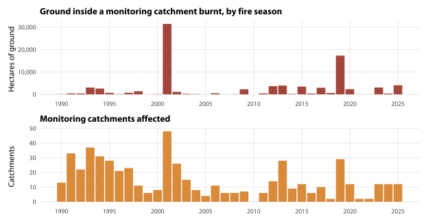
The upper panel needs one caveat spelled out, because it is easy to get wrong. The monitoring catchments nest: you deliberately pair small tributaries with the trunk streams they join, so a hectare of ground high in the Erskine or Kedumba catchment lies inside several monitoring catchments at once. Adding up burnt_ha across catchments therefore counts that hectare several times, and the result is not an area of land. The panel above measures the union instead — the ground inside any monitoring catchment that burnt — which is smaller, and not smaller by a constant factor. Summing across catchments would put 2001–02 at 51,785 ha rather than 31,472 ha and 2023–24 at 9,213 ha rather than 3,051 ha, which moves 2023–24 from the 3rd-largest season since 1990 to the 7th. The lower panel — the count of catchments affected — is unaffected by nesting and is the more directly interpretable of the two.

4.4.3.1 The 2019–20 Black Summer fires and the reference sites

This is the most consequential finding in the chapter, and it is a problem statement rather than a measurement: this section establishes that the benchmark moved. Section 14.4.1 measures how far, and chapter 14 owns that number. Do not quote a size of effect from here.

Table 4.16: The 19 monitoring catchments with at least 10% of their area burnt in the 2019-20 season, one row per catchment — one of them carries more than one monitoring point, and every site code on the catchment is listed.

Site(s)	Waterway	Tier	Catchment (ha)	% burnt	Fire(s)
01CMW	Waterfall Creek	Slightly disturbed	79	100	Gospers Mountain
02GBLR	Jungaburra Brook	Reference	64	100	Gospers Mountain
05.2GMVR	Asgard Brook	Reference	84	100	Grose Valley
05GMVR	Asgard Brook	Reference	129	100	Grose Valley
60GBLR	Pierces Pass Creek	Reference	182	100	Gospers Mountain
75BKTR	Reedy Creek	Reference	1870	100	Erskine Creek Fire
K53	Fortress Creek	Reference	21	100	Grose Valley
W14	Bennett Gully	Reference	1	100	Grose Valley
53BMGR	Breakfast Creek	Reference	349	100	Ruined Castle
54BMGR	Cedar Creek	Reference	3764	91	Ruined Castle
04GMV	Grose River tributary	Slightly disturbed	142	78	Grose Valley
06GBH	Hat Hill Creek	Slightly disturbed	146	62	Grose Valley
68EHZ	Corinne Creek	Urban	118	43	Riches Av, Woodford
79EGK	Erskine Creek	Slightly disturbed	20283	42	Red Ridge Fire Trail; Erskine Creek Fire; Riches Av, Woodford
M19	Garnett Creek	Urban	80	34	Riches Av, Woodford
11BMG	Megalong Creek	Urban	3670	33	Ruined Castle
03BMV	Fairy Dell Creek	Slightly disturbed	133	31	Grose Valley
32.2EWD, 32EWD	Garnett Creek	Urban	87	31	Riches Av, Woodford
73BKT	Kedumba River	Urban	7906	16	Cliff Dr, Katoomba; Ruined Castle; Erskine Creek Fire

9 of the 15 reference catchments that could be delineated were burnt over more than 90% of their area in 2019–20 (Table 4.16): 02GBLR, 05.2GMVR, 05GMVR, 53BMGR, 54BMGR, 60GBLR, 75BKTR, K53, W14. The Gospers Mountain and Grose Valley fires accounted for most of this, with the Ruined Castle and Erskine Creek fires making up the remainder. A further two reference catchments (28EHZR and 28.2EHZR, Ingar Dam and Ingar Creek) were only lightly touched in 2019–20 but had been burnt almost entirely in 2013–14.

Five reference catchments were burnt over more than half their area twice within seven years — in 2013–14 and again in 2019–20: 02GBLR, 05.2GMVR, 05GMVR, 60GBLR, W14. They are the top 5 rows of Figure 4.9, each carrying a dark cell in both seasons. That is five of the 15 delineated reference catchments, and it is the count the rest of the report should quote.

Table 4.17: Every reference catchment and fire season since 2000 in which more than 2% of the catchment burnt: 44 catchment-seasons at 15 reference catchments over 13 seasons, naming 25 distinct fires between them. The row is a catchment-season and not a fire — a season can bring more than one fire to one catchment, which is why the last column is plural. A blank in Fire(s) is not a missing row but a missing NAME — six of the 44 rows carry a recorded burn that the NPWS layer gives no fire name, all of them 2001-02.

Site	Waterway	Season	% of catchment burnt	Fire(s)
02GBLR	Jungaburra Brook	2006-07	79	Lawsons Long Alley
02GBLR	Jungaburra Brook	2013-14	98	Mount York Road; State Mine
02GBLR	Jungaburra Brook	2019-20	100	Gospers Mountain
05.2GMVR	Asgard Brook	2006-07	100	Lawsons Long Alley
05.2GMVR	Asgard Brook	2013-14	100	Mount York Road
05.2GMVR	Asgard Brook	2019-20	100	Grose Valley
05GMVR	Asgard Brook	2006-07	100	Lawsons Long Alley
05GMVR	Asgard Brook	2013-14	100	Mount York Road
05GMVR	Asgard Brook	2019-20	100	Grose Valley
28.2EHZR	Ingar Creek	2001-02	100
28.2EHZR	Ingar Creek	2013-14	95	Mount Bedford
28.2EHZR	Ingar Creek	2019-20	3	Erskine Creek Fire
28.2EHZR	Ingar Creek	2025-26	100	Mount Bedford
28EHZR	Ingar Dam	2001-02	100
28EHZR	Ingar Dam	2013-14	97	Mount Bedford
28EHZR	Ingar Dam	2019-20	3	Erskine Creek Fire
28EHZR	Ingar Dam	2025-26	100	Mount Bedford
52NGKR	Campfire Creek	2001-02	100
52NGKR	Campfire Creek	2017-18	18	HAW Campfire Creek HR
52NGKR	Campfire Creek	2023-24	73	Ironbarks Demonstration Burn; Red Hands Cave HR
53BMGR	Breakfast Creek	2003-04	37	Carlons Head
53BMGR	Breakfast Creek	2019-20	100	Ruined Castle
54BMGR	Cedar Creek	2017-18	27	UMT LMZ Mount Solitary
54BMGR	Cedar Creek	2019-20	91	Ruined Castle
56NSPR	Western Creek	2001-02	100
56NSPR	Western Creek	2012-13	37	St Helena HR
56NSPR	Western Creek	2023-24	70	Western Ridge HR
60GBLR	Pierces Pass Creek	2006-07	96	Lawsons Long Alley
60GBLR	Pierces Pass Creek	2013-14	99	Mount York Road; State Mine
60GBLR	Pierces Pass Creek	2019-20	100	Gospers Mountain
75BKTR	Reedy Creek	2001-02	7
75BKTR	Reedy Creek	2009-10	12	Red Ridge Fire Trail; Jensens Farm; Spring Creek (Jensens West)
75BKTR	Reedy Creek	2012-13	23	Kedumba Wall; Kedumba Walls
75BKTR	Reedy Creek	2019-20	100	Erskine Creek Fire
K40	Woodford Creek Trib	2018-19	100	UMT Lawson Ridge 2
K43	Woodford Creek Trib	2006-07	2	Lawsons Long Alley
K43	Woodford Creek Trib	2012-13	77	Linden Ridge Stage 2
K43	Woodford Creek Trib	2024-25	86	Linden Ridge
K53	Fortress Creek	2001-02	9
K53	Fortress Creek	2002-03	99	Blackheath Glen; Mt Hay
K53	Fortress Creek	2019-20	100	Grose Valley
W14	Bennett Gully	2006-07	100	Lawsons Long Alley
W14	Bennett Gully	2013-14	100	Mount York Road
W14	Bennett Gully	2019-20	100	Grose Valley

Figure 4.9: Fire in the reference catchments since 2000, one row per catchment and one column per fire season, each cell shaded by the share of the catchment’s area that burnt. This is the same set of catchment-seasons Table 4.17 lists — that table carries the fire names, which are the audit trail for the attribution, and this carries their shape. Read down the columns and three seasons separate themselves from the rest; read across the rows and the repeat burning the rating system has to cope with is immediate. Rows are ordered by how many seasons took more than half the catchment, so the catchments burnt over half their area in both 2013-14 and 2019-20 sit at the top with a dark cell in each, and the Ingar pair just below them shows the other pattern the text describes, burnt almost entirely in 2013-14 and barely touched in 2019-20. A blank cell is not ‘no fire’ but ‘no fire over 2% of the catchment’, which is the threshold the table uses.

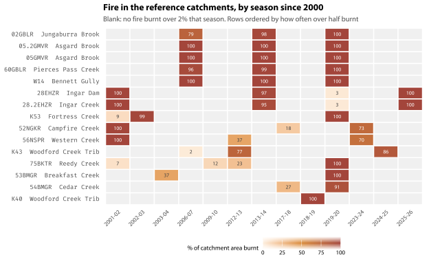
Why this matters for the rating system. The waterway health rating scores every stream sample twice: once against other Blue Mountains urban sites and once against reference sites. The reference bands were set from 2012–2015 percentile values. If reference streams were then burnt over almost their entire catchments in 2019–20 — after two of the four calibration years and following an earlier burn in 2013–14 — then:

• the reference bands describe a pre-fire reference condition that no longer exists in the field;
• a post-2020 sample at a reference site is being compared with its own pre-fire self, so a genuine fire effect will appear as a decline in reference condition, not as a change in urban streams;
• conversely, if the reference sites’ post-fire condition were used to re-derive the bands, urban sites would appear to improve for no reason at all.

How long the benchmark stays moved is not something these data can settle. The Australian evidence is more encouraging than the framing above implies: Robson et al. (2018) tracked five burnt and five unburnt headwater reaches in the Grampians through a 750 km² wildfire and found assemblages in the burnt streams indistinguishable from the unburnt ones within two years, with among-reach variability recovered within three. That is five reaches around one 2006 fire, in the middle of a twelve-year drought, and the paper’s own closing caution is that rising fire frequency may permanently alter the riparian vegetation headwater streams depend on. That is a reason to expect the reference benchmark to return rather than to be permanently lowered — but the Grampians fire was not followed by two of the wettest years on record, and chapter 14 measures what actually happened here.

Any chapter that reports a trend spanning 2019–20, and in particular the rating-system review, must treat the fire as a competing explanation and use years_since_fire and prop_burnt_3y to test it. The 1,904 of 2,062 macroinvertebrate samples with a prior catchment fire (92.3%) are identified in site_fire_bug, and the 2,576 of 2,688 water quality samples in site_fire_wq. Use those two objects, not site_fire_samples, which stacks both databases and would give a combined count of 4,480 — a number that belongs to neither series. This is the trap set out at Section A.3.

4.4.4 How badly it burnt, not just how much

The fire covariates above measure extent — how much of a catchment burnt. They do not measure how hard it burnt, and a catchment 80% burnt at low severity is not the same catchment as one 80% burnt at high severity. NSW DCCEEW’s Fire Extent and Severity Mapping (FESM) supplies the missing axis: a raster per fire season classifying every burnt pixel as low (understorey burnt, canopy intact), moderate (partial canopy scorch), high (full scorch, partial consumption) or extreme (full canopy consumption). 3,894 rows covering 11 seasons, 2013-14 to 2024-25, are held in fire_severity_catchment, one per catchment per season per zone.

Read the class lookup, do not read the raster values. FESM ships as two product families whose codes disagree on the value 1. In the operational series, from 2016–17 onward, 1 is reserved for future development — an unclassified placeholder. In the historical series, which covers 2013–14 and 2014–15, 1 is burnt grassland — a burn, but one with no canopy and so with no place on the four-step severity ladder. Pooling the two without recoding would count a placeholder as a burn in one half of the record and a burn as a placeholder in the other. The build reads the lookup that ships with the rasters rather than inferring classes from the values; over the monitoring catchments the two classes between them cover 0.0 ha of ground, so here the trap costs nothing — but that is a fact about this window, not about the data.

FESM and the NPWS extent layer do not map the same fires, and this bounds everything below. The historical series ships a hazard-reduction raster alongside the wildfire one, so 2013–14 and 2014–15 see prescribed burns. In 2013–14 the two products rank the catchments almost identically — Spearman 0.91 across 120 catchments. 2014–15 is a much smaller season, 4 catchments burnt in FESM against 9 in NPWS, and the agreement there is weaker, at 0.49. The operational series does not. From 2016–17 FESM is in practice a wildfire product, and the seasons from 2021–22 on are the clearest case: NPWS records fires in 22 catchment-seasons — spread across 4 distinct fire seasons — in which FESM maps nothing anywhere in the monitoring catchments, and almost all of those NPWS records are prescribed burns. A severity covariate of zero therefore does not always mean the catchment did not burn. Where it matters — 2013–14 and 2019–20, the two seasons that carry the signal — both products cover the fire. 2019–20 is wildfire, which is what the operational series maps, and there the two rank together again: Spearman 0.77 across the same 120 catchments. That is the ground the analysis stands on.

Table 4.18: Monitoring catchments carrying each FESM severity class in the two seasons that matter, out of 120 delineated catchment groups. Columns are counts of catchments with any of that class, with more than 1% of their area in it, and with more than 10%.

Season	Class	Any	>1%	>10%	Largest share of one catchment
2013-14	Low	32	26	16	80%
2013-14	Moderate	28	21	16	88%
2013-14	High	26	16	11	70%
2013-14	Extreme	11	9	0	9%
2013-14	High or extreme	26	17	11	72%
2019-20	Low	35	24	8	27%
2019-20	Moderate	36	21	14	74%
2019-20	High	22	17	11	80%
2019-20	Extreme	25	13	6	42%
2019-20	High or extreme	25	18	12	82%

How much severity signal is actually there. 54 of the 120 catchment groups burnt at all in the FESM record; 21 were burnt at high or extreme severity over more than a tenth of their area in some season, and 13 over more than a quarter. That is the number to hold on to, because it bounds every severity result in this report: across the whole FESM record the high-severity gradient is carried by 21 catchment groups, not by a hundred and twenty — and fewer than that reach the fitted analysis set (Section 4.4.4.1). The two seasons are also different in character rather than just in size. 2019–20 put 6 catchments over a tenth extreme where 2013–14 put 0 (Table 4.18); the October 2013 fires burnt widely but comparatively lightly, and the Black Summer fires burnt widely and hard.

Resolution. The historical series and the 2016–17 raster are ~30 m; from 2017–18 onward FESM is ~10 m. Every fraction here is computed from areas rather than pixel counts, so a fraction means the same thing on either grid, but the precision does not: the smallest catchment resolves to 29 cells on the 30 m grid against 175 on the 10 m grid. n_cells_zone travels with every row so that a fraction resting on a handful of pixels can be recognised as one.

Riparian corridors. Stream macroinvertebrates respond to what burns on the bank far more directly than to what burns on a ridge four kilometres upstream, so the same statistics are computed over a 30 m and a 100 m buffer around the mapped watercourses inside each catchment, in the same table under zone == "riparian_30m" and zone == "riparian_100m". Section 13.5.6 tests all three zones against the rating; the short answer is that in these catchments the corridor and the catchment burnt together, so the corridor carries almost the same number.

4.4.4.1 Severity, not just extent

Burnt fraction treats a catchment burnt at low severity and one burnt at extreme severity as the same catchment. That is testable: a severity term should beat an extent term on the same samples, or extent is the right measurement and the question closes. The set is the 730 edge stream samples at 77 sites, 2013–2024, carrying both measurements, so every model below is fitted to identical rows and the AICs are comparable. All carry a site and a year random effect.

Table 4.19: Fire measured as extent and as severity, against the published rating. All models fitted by maximum likelihood to the same 730 samples with a site and a year random effect. Estimates are points of avg_factor_score for a covariate moving from 0 to 1; negative means the rating falls.

Model	Term	AIC	Δ AIC	Estimate	t
No fire term	1	1320.3	10.0	—	—
Burnt fraction, NPWS extent	prop_burnt_3y	1314.6	4.3	-0.28	-2.80
Burnt fraction, FESM extent	fesm_burnt_3y	1312.3	2.0	-0.34	-3.20
High or extreme fraction, catchment	fesm_severe_3y	1310.3	0.0	-0.76	-3.48
High or extreme fraction, 100 m corridor	fesm_severe_3y_rip100	1310.6	0.2	-0.72	-3.44
High or extreme fraction, 30 m corridor	fesm_severe_3y_rip30	1311.4	1.1	-0.73	-3.32
FESM extent and severity together	fesm_burnt_3y + fesm_severe_3y	1311.3	0.9	-0.16, -0.54	-1.04, -1.76
NPWS extent and FESM severity together	prop_burnt_3y + fesm_severe_3y	1311.8	1.5	-0.09, -0.63	-0.70, -2.19

Severity wins, and extent does not survive beside it. The high-or-extreme burnt fraction of the catchment is 4.3 AIC better than the burnt fraction the NPWS extent layer supplies, and 10.0 better than no fire term at all (Table 4.19). Put the two in one model and the severity term keeps its size while the extent term collapses to -0.09 points with a t of -0.70. Extent adds nothing once severity is in the model.

The decisive test. Restrict to the 110 samples at 24 catchments where more than 5% of the catchment burnt in the previous three years, put the burnt fraction in the model, and add the share of that burnt area that burnt at high or extreme severity. Catchment area divides out of both ends of a share, so this term cannot be an extent effect wearing a different name. A catchment whose burn was entirely severe scores lower than one of the same size whose burn was entirely low-severity — 1.19 score points, 95% CI 0.49 to 1.90, p = 0.002 on a likelihood-ratio test, over 110 samples at 24 catchments from 2014 to 2023.

That interval is narrower than the design can support, which is why it is not set beside the rating class width here. Severity share is a property of the catchment, not of the sample: it varies 0.19 between sites against 0.05 within them, and twelve of the 24 sites show no within-site variation in it at all. The 110 samples above are therefore not 110 independent readings of severity share, and an interval computed as though they were is too narrow. Fitted at the level the predictor actually varies at — one row per site, 24 of them — the same contrast is 1.27 points, 95% CI -0.41 to 2.96, p = 0.13, which does not separate from zero. For scale a rating class is 1.00 score points wide, so that interval spans -0.41 to 2.96 rating classes — which is why the earlier claim that severity costs “about a full rating class” is withdrawn here rather than restated with a wider interval.

Read that as a direction, not as a coefficient. It rests on 24 catchments, and the interval is wide because that is how many there are. The finding is severity matters and extent does not — which the model comparison supports on its own terms — and it is not precise enough to be anything more. In particular it does not support “about a full rating class”, which is what this passage used to claim.

Table 4.20: The severity-share effect under four specifications, each with the burnt fraction and both random effects also in the model. Estimates are points of avg_factor_score between an entirely low-severity burn and an entirely severe one; negative means the rating falls.

Specification	Estimate	SE	t	n
As above	-1.19	0.36	-3.30	110
Plus climate state (SPI-12, log 30-day rain)	-0.99	0.38	-2.59	110
Plus disturbance tier	-1.00	0.36	-2.78	110
Severity share of the 100 m riparian corridor	-1.29	0.36	-3.54	110

The effect is not one catchment and it is not the year term. Dropping each of the 18 catchments that carry a severity share above 0.10 in turn leaves it between 0.96 and 1.87 points, always in the same direction. Removing the year random effect strengthens it to 1.40, which is the opposite of the pattern that would appear if a network-wide good year were being charged to the lightly burnt catchments.

And it is not a before-and-after, which matters here more than usual. The Black Summer fire is followed immediately by the wettest run of years in the record, by an instrument change and by a shift in flow state, so anything measured across 2020 is confounded three ways by construction. This is a comparison across catchments within the same year — creeks that burnt at different severities, sampled in the same years, by the same officers, with the same probe. The year random effect removes the between-year contrast entirely, so that within-year spread is all the estimate is fitted to, and it is real: in 2020, 13 burnt catchments were read whose severity shares ran from 0.00 to 0.82.

The 2013–14 fires on their own, which are worth separating precisely because they are not next to 2020. On the 229 samples from 2014 to 2017 at 61 sites, both extent measures are flat while the severity term points the same way as the pooled estimate and about as far (Table 4.21).

Table 4.21: Fire and the rating in the 2014-2017 window, which the 2013-14 fires dominate and which no part of the 2020 confound reaches. 229 samples at 61 sites; 9 catchments carry a high-severity fraction above 10%. p is against a model with no fire term.

Term	Estimate	SE	t	p
prop_burnt_3y	0.04	0.18	0.22	0.830
fesm_burnt_3y	0.04	0.18	0.24	0.816
fesm_severe_3y	-0.76	0.65	-1.18	0.246

It does not reach significance, and on 9 catchments carrying a high-severity fraction it was never going to. What it rules out is the reading that the pooled result is an artefact of 2020: in the one window no part of the 2020 confound reaches, and where extent has no explanatory power at all, severity has the same sign and roughly the same size as it does overall.

The riparian corridor adds nothing, and the reason is in the fires themselves. Corridor and whole-catchment severity correlate at 0.99 here. These fires burnt catchments whole — nothing in the network burnt severely on its ridges and lightly on its banks — so there is no contrast for a riparian covariate to exploit. The corridor statistics are built and waiting; in a fire with a different footprint they would be the more mechanistic covariate, but on this record they are the catchment number measured twice.

What bounds it. 13 catchments in this set carry a high-or-extreme fraction above a tenth, against 25 carrying a burnt fraction above a tenth. The severity gradient is the thinner of the two, which is what makes it notable that it is also the stronger predictor and is why the interval is wide. The severity classification is a remote-sensing product with its own error, not propagated into any interval here. And Section 4.4.4’s coverage caveat applies: because FESM maps few prescribed burns after 2016–17, a handful of samples here are recorded as unburnt by FESM and burnt by NPWS — which works against the severity term, not for it.

4.5 What this chapter cannot do

The data-availability half of this list is at the top of the chapter, as questions. What is left is analytical — things no further data request fixes — with two exceptions, marked as such at items 3 and 9. Both are restated here because until the answers arrive they bind exactly as hard as the seven that no answer would move.

1. Imperviousness is part measured and part modelled, and it has not been validated. Roof area is measured; the paving that goes with it, the sealed fraction of a road corridor and the conversion to a connected figure are not. The comparison against your own tiers in Section 4.3.6 is a consistency check, and it cannot test the conversion at all. Use it as a ranking, report it as modelled, and do not treat the 5% line as discriminating — Section 4.3.3.4 is the third independent reason for that.

2. What is still assumed is the paving, not the roof, and the reported bounds are a scenario range, not a confidence interval. Roof area is measured, not modelled, since 29 August 2026: method ST’s premises term is Council’s Geoscape roof area, the same layer Section 4.3.7 uses, and ti_primary is built on it. The 239,073 open building footprints covering the study window (Section 4.3.4) are held too, but they are not what it reads. The paving multiple sets the level in residential catchments; dci_lo and dci_hi vary that (halved and doubled), the road sealed fraction (35–55%) and Sutherland’s connection class, and nothing else. They span none of the larger sources of spread — the choice between the three imperviousness methods, or the pour-point rule — and the land-use and mesh-block estimates fall inside the band for only 35 and 13 of the 120 catchments.

3. 8 of the 137 register sites are withheld from delineation, so they have no catchment, no imperviousness and no site-specific climate; they take the regional mean climate and are flagged. Their candidate positions are far enough apart to give materially different catchments and averaging two plausible positions produces a third that is wrong with certainty. Every register site does hold an easting and a northing — this is an ambiguity about which position is right, not a gap. One of the two items here that a data request does fix: dq:site-coords-ambiguous asks which candidate is right, site by site. (The candidate spreads are deliberately not repeated here: they live in SITE-SUBSETS.md and on that question, not on the targets graph.)

4. 51 of the 120 catchments are rated moderate or low confidence, and 18 of the 120 imperviousness estimates are rated low. They are flagged in site_catchments rather than hidden, and a sensitivity check excluding them is cheap. Read the grade literally: it says the catchment area does not depend on which snapping rule we used, which is a claim you can act on.

5. The drainage network we can trace is 20.3% of the one that exists (Section 4.3.3.2). That bounds the connected-imperviousness test in Section 4.3.7, and it is the reason the answer there is about what you can currently measure rather than about connectivity as a concept.

6. Land use covers 100.0% of every catchment (0 under 99%), so the numbers in Section 4.3 are computed on all 120 of them, and none of the catchments is scored on a partial layer. The structural estimate, the modelled figures and the catchment areas do not read that layer at all.

7. SILO is an interpolated surface, not a gauge. Its 0.05 degree grid cannot resolve orographic rainfall gradients within a few kilometres, which in the upper Mountains are real. Antecedent rainfall is a good relative index, not a measurement at the site.

8. Fire severity rests on thirteen catchments. The covariates exist and they work (Section 4.4.4.1), but the high-severity gradient is carried by 13 catchments in the analysis set, not by a hundred and twenty. The larger figure quoted at Section 4.4.4 belongs to a different population: 21 catchment groups carry a high-or-extreme fraction above a tenth somewhere in the FESM record, and 13 of them are in the analysis set. Treat it as a direction, not as a coefficient.

9. No treatment evaluation is possible without commissioning dates and designated controls, as set out in Section 17.3. The second of the two items a data request does fix. The dates are held in Council’s asset records rather than absent from the world, and dq:sqid-commissioning-dates asks for them.

Sources

Full download provenance — source, URL, date, size and licence for every external dataset — is recorded in R/data/external/MANIFEST.md, which is committed to the repository even though the data files themselves are not.

Table 4.22: The 9 external datasets used in this chapter, with the full download provenance for each in R/data/external/MANIFEST.md. Council-supplied layers are deliberately not listed here — the 12 m DEM_Broadscale surface, the stormwater asset register, the 2003 first-order catchment polygons and the Geoscape building footprints behind both the structural estimate in Section 4.3.4 and the traced connected estimate in Section 4.3.7 all come from you rather than from a public source, and their provenance is in R/data/council-gis/MANIFEST.md.

Dataset	Custodian	Licence
1 Second SRTM Hydrologically Enforced DEM (DEM-H) v1.0	Geoscience Australia (via Digital Earth Australia)	CC BY 4.0
SILO Data Drill daily climate surfaces	Qld Department of Environment, Science and Innovation	CC BY 4.0
NPWS Fire History — wildfires and prescribed burns	NSW DCCEEW (via SEED)	CC BY 4.0
Fire Extent and Severity Mapping (FESM) and Historical FESM	NSW DCCEEW (via SEED)	CC BY 4.0
NSW Landuse 2017 v1.5	NSW DCCEEW (via SEED)	CC BY 4.0
Digital Cadastral Database — road corridor polygons	NSW Spatial Services	CC BY 4.0
NSW Geocoded Addressing Theme — address points	NSW Spatial Services	CC BY 4.0
Mesh Blocks, ASGS Edition 3 (2021)	Australian Bureau of Statistics	CC BY 4.0
Microsoft GlobalMLBuildingFootprints — open building footprints	Microsoft (AI-derived, Australia partition)	CDLA Permissive 2.0

Key references. The works cited in this chapter are listed in full in the References at the end of the book, together with the rest of the report’s bibliography.

Booth, Derek B., and C. Rhett Jackson. 1997. “Urbanization of Aquatic Systems: Degradation Thresholds, Stormwater Detection, and the Limits of Mitigation.” Journal of the American Water Resources Association 33 (5): 1077–90. https://doi.org/10.1111/j.1752-1688.1997.tb04126.x.

Davies, Peter J., Ian A. Wright, Sophia J. Findlay, Olof J. Jonasson, and Shelley Burgin. 2010. “Impact of Urban Development on Aquatic Macroinvertebrates in South Eastern Australia: Degradation of in-Stream Habitats and Comparison with Non-Urban Streams.” Aquatic Ecology 44 (4): 685–700. https://doi.org/10.1007/s10452-009-9307-y.

Gallant, John, Nicholas Wilson, Trevor Dowling, Arthur Read, and Craig Inskeep. 2011. SRTM-Derived 1 Second Digital Elevation Models Version 1.0. Dataset, Geoscience Australia, Canberra. https://data.gov.au/dataset/ds-dga-9a9284b6-eb45-4a13-97d0-91bf25f1187b.

Gomez Isaza, Daniel F., Rebecca L. Cramp, and Craig E. Franklin. 2022. “Fire and Rain: A Systematic Review of the Impacts of Wildfire and Associated Runoff on Aquatic Fauna.” Global Change Biology 28 (8): 2578–95. https://doi.org/10.1111/gcb.16088.

Hack, John T. 1957. Studies of Longitudinal Stream Profiles in Virginia and Maryland. Professional Paper 294-B. U.S. Geological Survey. https://doi.org/10.3133/pp294b.

Hatt, Belinda E., Tim D. Fletcher, Christopher J. Walsh, and Sally L. Taylor. 2004. “The Influence of Urban Density and Drainage Infrastructure on the Concentrations and Loads of Pollutants in Small Streams.” Environmental Management 34 (1): 112–24. https://doi.org/10.1007/s00267-004-0221-8.

McKee, Thomas B., Nolan J. Doesken, and John Kleist. 1993. “The Relationship of Drought Frequency and Duration to Time Scales.” Proceedings of the 8th Conference on Applied Climatology, 17–22 January 1993, Anaheim, California (Boston), 179–84. https://climate.colostate.edu/pdfs/relationshipofdroughtfrequency.pdf.

Robson, B. J., E. T. Chester, T. G. Matthews, and K. Johnston. 2018. “Post-Wildfire Recovery of Invertebrate Diversity in Drought-Affected Headwater Streams.” Aquatic Sciences 80 (2): 21. https://doi.org/10.1007/s00027-018-0570-7.

Sutherland, R. C. 2000. “Methods for Estimating the Effective Impervious Area of Urban Watersheds.” Chap. 32 in The Practice of Watershed Protection, edited by Thomas R. Schueler and Heather K. Holland. Center for Watershed Protection. https://yourcleanwater.org/wp-content/uploads/2021/10/CWP-Sutherland-DCIA-Paper.pdf.

Verkaik, Iraima, Maria Rieradevall, Scott D. Cooper, John M. Melack, Tom L. Dudley, and Narcís Prat. 2013. “Fire as a Disturbance in Mediterranean Climate Streams.” Hydrobiologia 719 (1): 353–82. https://doi.org/10.1007/s10750-013-1463-3.

Walsh, Christopher J., Tim D. Fletcher, and Anthony R. Ladson. 2005. “Stream Restoration in Urban Catchments Through Redesigning Stormwater Systems: Looking to the Catchment to Save the Stream.” Journal of the North American Benthological Society 24 (3): 690–705. https://doi.org/10.1899/04-020.1.

Walsh, Christopher J., and Joshphar Kunapo. 2009. “The Importance of Upland Flow Paths in Determining Urban Effects on Stream Ecosystems.” Journal of the North American Benthological Society 28 (4): 977–90. https://doi.org/10.1899/08-161.1.

Walsh, Christopher J., Allison H. Roy, Jack W. Feminella, Peter D. Cottingham, Peter M. Groffman, and Raymond P. Morgan. 2005. “The Urban Stream Syndrome: Current Knowledge and the Search for a Cure.” Journal of the North American Benthological Society 24 (3): 706–23. https://doi.org/10.1899/04-028.1.