10  The rare families, and what a condition rating cannot see

Blue Mountains City Council Healthy Waterways — statistical analysis

10.1 A rating cannot see this, and that is the point

A waterway health rating measures condition — how degraded a creek is relative to other creeks. It is good at that, and it should be kept. But condition and conservation value are different things, and an index built to measure the first is structurally incapable of measuring the second.

The four current factors treat every family alike. A stonefly of the family Eustheniidae — one of the largest and most sensitive animals in the Australian freshwater fauna — counts for exactly as much as a chironomid midge: one family each. SIGNAL-SF has no grade at all for 11 of the 42 rare families here. The %EPT and EPT-family factors catch some of the sensitive rare taxa and miss the dragonflies, lacewings, toe-winged beetles and crane flies that carry the same signal. A creek can rate Fair and be the most important creek in the network, and nothing in the score will say so.

So this chapter is not a driver ranking. It is one argument, in three steps:

42 families are recorded in fewer than 20 of the 1,502 samples, and they are two groups that want opposite things. Averaging them destroys the signal, which is why nobody has seen it.

The rare families as a whole are declining, at -29% per decade once every sample is rarefied to a constant 50 animals — effort removed by construction rather than modelled away.

What is left is concentrated in ten named creeks, most of which are not reference sites, plus one established population of a restricted amphipod. Those are things you can protect, and a condition rating will never point at them.

Nobody asked for this section. It is the part of the report most likely to change what actually gets done.

10.1.1 What this chapter will and will not bear

Table 10.1: What this chapter answers, and how much weight each answer will bear.

Question	Answer	How much weight it bears
What is special about the sites that hold rare families?	It depends which rare families, and that is the finding. The sensitive ones want coarse, unsilted beds, larger catchments and well-oxygenated water, but false-discovery-rate control across the 18 predictors leaves one: catchment area. Fine sediment, dissolved oxygen, imperviousness and alkalinity all point the same way and none of them survives it. The rest are lowland still-water animals, rare here because the Blue Mountains are steep and cold.	Moderate to high for the direction, low for the magnitudes — 65 occurrences of sensitive rare families in the whole record.
Are rare families being lost?	Yes. -21% per decade per sample and -30% on the panel monitored in twelve or more years, with the effort artefact running the other way; and -29% (-44% to -8.3%, p = 0.008) with effort removed by rarefaction rather than modelled.	High for the direction, which is negative at all six threshold fits and conservative against the one bias in the data — but four of the six reach significance, not all of them: at the lowest cut, fewer than 15 samples, where the rare set is smallest and the counts sparsest, the interval includes zero on both sample sets (Section 10.4.2). Moderate for the rate, which is not precise.
Are the sensitive rare families falling faster?	On the threshold used here, yes — -48% per decade on the panel. At a cut of 30 samples it does not fall at all (+13%, p = 0.39).	Low. This is the one number in the chapter a reviewer can overturn by moving a cutoff, and Section 10.4.2 shows exactly how. Argue the case from the all-rare decline instead.
Which creeks should be protected?	The ten that have recorded more than one sensitive rare family, plus Waterfall Creek for its Paramelitidae population. Below those, 29 sites hold exactly one and cannot be separated from each other.	Moderate to high for the named sites; high for the statement that a longer list is reporting a tiebreak as a rank, which the bootstrap in Section 10.5 settles.
Should rare families go into the rating?	No. A rare-family bonus would change about 1% of ratings, because most samples hold no sensitive rare family at all. A flag on the site record is the right instrument.	High. This is arithmetic on the zero-inflation, not a modelling judgement.

10.2 The data behind this chapter

Each question and request below is set out again in What we need from you, with what it blocks, what an answer is worth and what it would cost you to find, ranked against every other ask in the report.

10.2.1 What this chapter uses, and where it came from

Every other number in this chapter comes from edge samples only. The Paramelitidae records are counted over the whole archive, riffle samples included, and that is on purpose.

Where an animal has been found is a conservation claim, not an analysis result, so restricting it to the edge-only set would understate how scattered the isolated detections are. One of the records is a 2006 riffle sample at a third creek, which the edge-only set drops — and that record is exactly the kind of thing a protection decision needs to know about. It is flagged in the table’s caption (Table 10.8) as well, so nobody reconciles the two counts and concludes one of them is wrong.

Blocks: Nothing — this is a statement of what we did. Value: moderate. Costs you: minutes. Refer to it as dq:paramelitidae-counted-over-archive.

A family counts as rare in this chapter if it appears in fewer than 20 of the edge stream samples. That line has to be drawn somewhere, so it is drawn at 20 and then redrawn at 15 and at 30 to see what moves.

Twenty is where family-by-family testing runs out of power — below it, no single family can carry a test of its own. The rare set is built from the same analysis set as the rest of Part II: edge habitat, family-level identifications, microfauna dropped, streams only. Sensitivity is a SIGNAL 2 grade of 6 or higher, or membership of the mayfly, stonefly or caddisfly orders. Everything in the chapter that depends on the threshold is refitted at all three cuts, and the results are in the chapter rather than in a footnote.

Blocks: Nothing — this is a statement of what we did. Value: moderate. Costs you: minutes. Refer to it as dq:rare-set-definition.

10.2.2 What is wrong with it

Nothing in this chapter can distinguish a family that was absent from one that was present and not picked out of the tray, and for animals recorded two or three times in a quarter century that distinction is most of the uncertainty.

Every model here carries the log number of animals counted as an effort proxy, and the rarefied analysis removes effort by construction, which is as far as this design can go. What it cannot do is estimate a detection probability, because that needs repeat samples within a season at the same site — which the program does collect occasionally, and which nobody has catalogued. The intervals in this chapter are wide for a real reason and should not be narrowed by wishful reading.

Blocks: Any per-family statement; occupancy modelling with a detection sub-model. Value: moderate. Costs you: minutes. Refer to it as dq:absence-versus-non-detection.

Two of the rare families carry no order in the taxonomy table and no SIGNAL grade of either kind, so the sensitivity rule cannot see them and they fall into the “other” group by default rather than by evidence.

They are shown as “unplaced” in the rare-family table (Table 10.2). It is a small number and it does not change the group contrast, but it is a default, not a finding, and a reader is entitled to know which way it was defaulted. Separately, six taxon names in the archive do not match the taxonomy after normalisation — two of them are among the families this chapter would otherwise call lost, which is why three of the twelve apparent losses are discounted before the pattern is claimed.

Blocks: A clean sensitive/other split, and a clean count of families lost. Value: moderate. Costs you: an afternoon. Refer to it as dq:unplaced-families-no-grade.

10.2.3 Questions only you can answer

When did each family name enter or leave the laboratory’s reference list? A dated version of the list would be ideal — failing that, does anyone remember Antipodoeciidae turning up?

The report’s headline conservation finding is that twelve rare families disappeared before 2011, and three of those have already turned out to be nomenclature rather than extinction. The 48% decline in sensitive rare families is not robust to where the rarity threshold is drawn, and the families that reverse it look like list changes: Antipodoeciidae has 24 of its 26 records after 2011 and none before 2006. This is the last open attack on the most consequential conservation claim in the report, and the reference list is what closes it.

Refer to it as dq:dated-family-list.

10.2.4 What would answer them

Could the Waterfall Creek Paramelitidae get a specialist identification? And is the field sheet for sample 590 (2010, 100 individuals) still around to confirm that count?

This is the named high-conservation-value population in the report and a protection recommendation rests on it. Unlike most of this list it is new expert work rather than a filing-cabinet search, so it costs real money — but it is a small amount of money against the weight the finding carries.

Refer to it as dq:paramelitidae-verification.

10.3 Two kinds of rarity, and why the split matters

10.3.1 How rarity is distributed

Rarity has two dimensions and they are not the same thing. A family recorded at one site in most years is rare in a completely different way from one recorded once at each of a dozen sites: the first is a restricted population that could be protected, the second is a wanderer that is probably common somewhere else.

Figure 10.1: Occupancy of the 117 macroinvertebrate families, in samples and in sites. The 42 families to the left of the dashed line are recorded in fewer than 20 of the 1,502 samples and are the rare set analysed here. Families near the diagonal appear once at each of several sites; families well below the diagonal, such as the freshwater amphipod Paramelitidae, are concentrated at very few sites and are the ones with a genuine conservation claim.

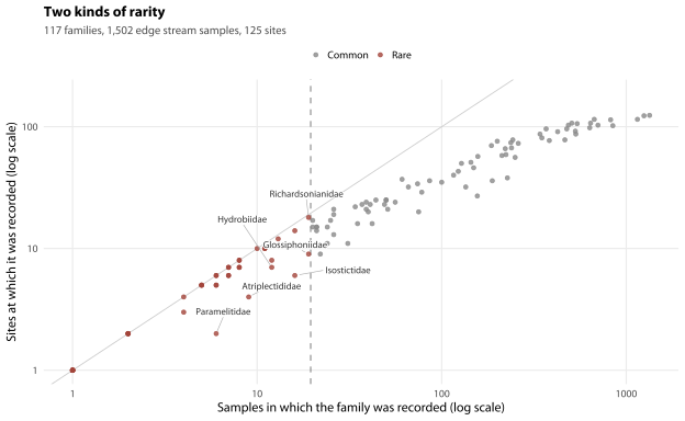
42 of the 117 families are recorded in fewer than 20 of the 1,502 samples. Together they account for 279 occurrences, 1.5% of all family records, and 22 of them are found at five sites or fewer.

Why 20 samples? Partly because it is where chapter 8’s family-by-family tests run out of power — below it, no single family can carry a test of its own. But a threshold chosen for one chapter’s convenience is not a reason, so Section 10.4.2 refits everything at 15, 20, 30 and reports what moves. Read the two together: the definition is arbitrary, and the result that matters does not depend on it.

These 42 families are not one group, and treating them as one produces a misleading answer, and Table 10.2 is the split. 13 of them are sensitive animals — mayflies, stoneflies, caddisflies, damselflies and dragonflies, aquatic lacewings, a toe-winged beetle, a primitive crane fly and an amphipod, all with a SIGNAL 2 grade of 6 or higher or membership of the mayfly, stonefly and caddisfly orders. The other 29 are mostly still-water and marginal animals — leeches, water bugs, snails, shore flies — which are rare in these creeks because these creeks are fast and cold, not because they are threatened.

Table 10.2: The 42 rare families, split by sensitivity. ‘Sensitive’ means a SIGNAL 2 grade of 6 or higher, or membership of the mayfly, stonefly or caddisfly orders. Two families have no order recorded in the taxonomy table and no SIGNAL grade; their Order reads ‘Unplaced’ and their grade is a dash.

Family	Common name	Order	Samples	Sites	SIGNAL 2	Group
Ameletopsidae	a predatory mayfly	Ephemeroptera	1	1	7	Sensitive
Eusiridae	an amphipod	Amphipoda	1	1	7	Sensitive
Oeconesidae	a caddisfly	Trichoptera	1	1	8	Sensitive
Osmylidae	lance lacewing	Neuroptera	1	1	7	Sensitive
Eustheniidae	a large stonefly	Plecoptera	2	2	10	Sensitive
Neurorthidae	an aquatic lacewing	Neuroptera	4	3	9	Sensitive
Glossosomatidae	saddle-case caddisfly	Trichoptera	5	5	9	Sensitive
Diphlebiidae	blue riverdamsel	Odonata	7	7	6	Sensitive
Tanyderidae	primitive crane fly	Diptera	7	6	6	Sensitive
Austrocorduliidae	a dragonfly	Odonata	8	7	10	Sensitive
Ptilodactylidae	toe-winged beetle	Coleoptera	8	8	10	Sensitive
Atriplectididae	a caddisfly	Trichoptera	9	4	7	Sensitive
Austroperlidae	a stonefly	Plecoptera	11	10	10	Sensitive
Erpobdellidae	a leech	Hirudinea	1	1	1	Other
Gomphomacromiidae	a dragonfly	Unplaced	1	1	–	Other
Limnichidae	minute marsh-loving beetle	Coleoptera	1	1	4	Other
Spercheidae	a water scavenger beetle	Unplaced	1	1	–	Other
Chaoboridae	phantom midge	Diptera	2	2	2	Other
Naucoridae	creeping water bug	Hemiptera	2	2	2	Other
Ornithobdellidae	a leech	Hirudinea	2	2	1	Other
Protoneuridae	threadtail damselfly	Odonata	2	2	4	Other
Ephydridae	shore fly	Diptera	4	4	2	Other
Hydridae	hydra	Hydrozoa	5	5	2	Other
Sciomyzidae	marsh fly	Diptera	5	5	2	Other
Ceinidae	an amphipod	Amphipoda	6	6	2	Other
Corbiculidae	a freshwater clam	Pelecypoda	6	5	4	Other
Hebridae	velvet water bug	Hemiptera	6	5	3	Other
Noteridae	burrowing water beetle	Coleoptera	6	6	4	Other
Paramelitidae	a freshwater amphipod	Amphipoda	6	2	4	Other
Chrysomelidae	leaf beetle	Coleoptera	7	7	2	Other
Phreatoicidae	a phreatoicid isopod	Isopoda	7	6	4	Other
Sialidae	alderfly	Megaloptera	8	7	5	Other
Staphylinidae	rove beetle	Coleoptera	8	8	3	Other
Curculionidae	weevil	Coleoptera	10	10	2	Other
Tabanidae	horse fly	Diptera	11	10	3	Other
Haliplidae	crawling water beetle	Coleoptera	12	8	2	Other
Hydrobiidae	a freshwater snail	Gastropoda	12	7	4	Other
Mesoveliidae	water treader	Hemiptera	13	12	2	Other
Isostictidae	narrow-winged damselfly	Odonata	16	6	3	Other
Pleidae	pygmy backswimmer	Hemiptera	16	14	2	Other
Glossiphoniidae	a leech	Hirudinea	19	9	1	Other
Richardsonianidae	a leech	Hirudinea	19	18	4	Other

10.3.2 What kind of site supports them

Raw rare-family richness cannot be modelled without an effort term. The number of families recorded rises with the number of animals counted, and a rare family is by definition the one most likely to be missed in a small sample, so every model below carries the log of the number of animals counted. Its coefficient is 0.86 — on a base-10 log scale against a natural-log link, which implies rare-family richness rising as roughly the 0.38 power of the count: doubling the number of animals picked out of the tray raises expected rare-family richness by about 30%. A purely mechanical detection effect would give an exponent of 1, so detection here is sub-proportional — but it is still much the largest nuisance in these models.

Each model is a Poisson mixed model with a site random effect, fitted to 1,245 samples at 75 sites, reporting the change in log rare-family richness per standard deviation of the predictor.

Figure 10.2: What predicts rare-family richness, fitted separately for the sensitive rare families and the rest. The two groups respond in opposite directions to almost everything; sensitive rare families increase where fine sediment is low and catchment imperviousness is low, while the other rare families increase where conductivity is high, riffle is scarce and altitude is low. Pooling them, as a single rare-family count would, cancels the two signals out. Filled points survive false-discovery-rate control across the 18 predictors tested for that response; open points do not. In the sensitive panel catchment area is the only filled point, and dissolved oxygen, fine sediment, alkalinity, and catchment imperviousness come nearest to surviving it and are all open. In the other-rare panel six points are filled - conductivity, altitude, riffle, macrophytes, alkalinity, and catchment area - which is more than the four the text describes as a lowland pool, and the text says which two it leaves out and why.

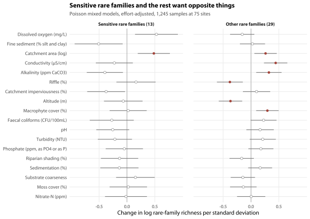
These are 54 models — 18 predictors against three responses — so the p-values need multiplicity control before any of them is named. The false discovery rate is controlled within each response by the Benjamini–Hochberg procedure (Benjamini and Hochberg 1995) over the 18 predictors, and the q-values below are what survives it.

The sites that support sensitive rare families are large-catchment reaches with coarse, unsilted beds and well-oxygenated water. Of the 18 predictors tested against sensitive rare-family richness, false-discovery-rate control leaves one: catchment area. Richness rises by 62% per standard deviation of catchment area (q = 0.02).

The rest of the picture points the same way and does not survive the correction; read it as suggestive rather than established. Each standard deviation of silt and clay in the substrate is associated with a 40% fall in sensitive rare-family richness (95% CI 7.4% to 61%, q = 0.09); richness rises by 70% per standard deviation of dissolved oxygen (q = 0.06); and it falls with catchment imperviousness (-31% per standard deviation, q = 0.11) and with alkalinity (-33%, q = 0.09). All four are on the same footing, and none of them is established. The imperviousness leg is the one to watch, because it is the leg that connects the rare families to your planning levers.

Fine sediment appearing among them at all is what the literature would predict, and that matters: the result rests on visual substrate estimates and could otherwise be read as an artefact of them. Deposited silt and clay fill the interstitial spaces coarse substrate provides, clog respiratory surfaces and displace the scrapers and shredders that dominate clean gravel beds (Wood and Armitage 1997). The relationship is real and widely reported, but it is not precisely quantified: Jones et al. (2012) open by calling the relationship between fine sediment and macroinvertebrate response poorly defined, which is the honest support for a by-eye substrate variable anyway. The sensitive rare families here are largely those same interstitial and coarse-substrate taxa. The provenance caveat still travels with it: substrate is estimated by eye, against no written protocol, and chapter 3 (Section 3.6.2) sets out what that costs. Fine sediment happens to be one of the better-behaved fields — the officer who wrote the sheet accounts for essentially none of its variance — but “estimated by eye” is the right label for it.

The other rare families give the opposite picture, and it is not a conservation signal: they are commoner where conductivity is high (0.44 per standard deviation), riffle is scarce (-0.38), altitude is low (-0.37) and macrophytes are abundant (0.29). That is a description of a slow, warm, weedy lowland pool. Those families are rare in the Blue Mountains because the Blue Mountains are mostly steep sandstone headwaters.

Those four are the four that fit that description. They are not all of what survives the correction, and Figure 10.2 draws the difference. Six of the 18 predictors clear false-discovery-rate control for this group — conductivity, altitude, riffle, macrophytes, alkalinity, and catchment area — at q = 0.032 or better. The two the habitat description leaves out point opposite ways at each other, and it is worth saying which. Alkalinity (0.32 per standard deviation) is the contrast again, because the sensitive group’s estimate for the same variable is -0.40. Catchment area is not. It is the one predictor that survives the correction for both groups, and it points the same way in both — 0.48 for the sensitive families, 0.26 for the rest. Bigger catchments hold more of both kinds of rare family, and that is the single place these two groups agree where the evidence is strong enough to say so at all. Everywhere else the correction can see, the contrast holds — and it holds against a sensitive group only one of whose own 18 predictors survives the same correction.

This is why a single rare-family count is the wrong metric. Pooled across all 42, imperviousness has no detectable effect at all (-0.02, CI -0.22 to 0.18), because the two groups cancel.

10.3.3 Borrowing strength across the 42 taxa

42 separate models on taxa recorded a handful of times each would be 42 underpowered tests. A hierarchical multi-species model fits all of them at once, with each family’s response drawn from a common distribution, so that a family recorded twice is informed by the families recorded twenty times.

It is not a joint species distribution model, and the distinction matters if anyone plans to build on it. The taxon-level effects here are independent by construction — diag() on the taxon random effects — and there is no latent term, so the model shares strength across families and says nothing about which families co-occur once the drivers are accounted for. Calling it a joint SDM would put a capability in the report that the code does not have. (It is also loose to call it an occupancy model, strictly: there is no detection sub-model, only detection/non-detection with effort as a fixed-effect proxy. “Hierarchical multi-species occurrence model” is the exact term.)

Table 10.3: Hierarchical multi-species occurrence model over all 42 rare families (52,794 family-by-sample rows, 230 presences, 1,257 samples). Each coefficient is the change in log-odds of a family being present per standard deviation of the driver. The third column is the difference in that response for the sensitive families; a large negative value means the sensitive families respond in the opposite direction to the rest.

Driver	Other rare families	Difference for sensitive	Net, sensitive	p
Altitude (m)	-0.35 (-0.53 to -0.16)	+0.75 (0.29 to 1.22)	+0.40	0.002
Catchment imperviousness (%)	+0.39 (0.12 to 0.66)	-0.47 (-0.95 to 0.01)	-0.08	0.057
Catchment area (log)	+0.27 (0.05 to 0.48)	+0.34 (-0.12 to 0.80)	+0.61	0.145
Fine sediment (% silt and clay)	+0.03 (-0.17 to 0.22)	-0.32 (-0.78 to 0.14)	-0.29	0.169
Macrophyte cover (%)	+0.27 (0.10 to 0.44)	-0.24 (-0.60 to 0.12)	+0.03	0.196
Riparian shading (%)	-0.01 (-0.23 to 0.20)	+0.21 (-0.20 to 0.61)	+0.19	0.317

The model confirms the split with one formal test rather than two separate regressions, and Table 10.3 is that test. Altitude is the clearest: the other rare families become less likely with altitude (-0.35 per standard deviation), while the sensitive families become 0.75 more likely per standard deviation than that (p = 0.002), so the net response for a sensitive rare family is +0.40. The differences for fine sediment (-0.32, p = 0.169) and imperviousness (-0.47, p = 0.057) point the same way with weaker evidence, which is what 230 presences across 42 taxa can support.

Figure 10.3: Each rare family’s own fitted response to fine sediment and to catchment imperviousness. The sensitive families cluster in the lower left — less likely to be present where the bed is silted and the catchment is sealed — and the other rare families in the upper right. The separation is the model’s answer to what makes a site special for rare taxa. Every point is shrunk towards its group mean, heavily so for the eight families recorded in a single sample.

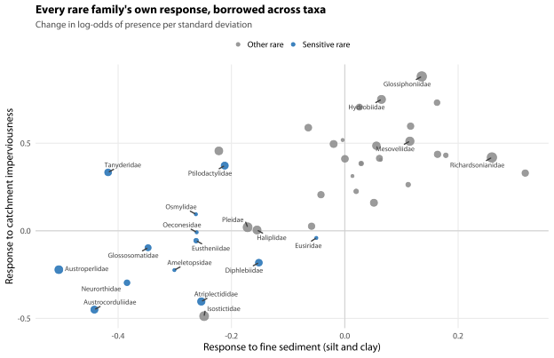
If you want the model that says which families co-occur, it is a different model and it has not been fitted. That needs a residual correlation structure — gllvm, Hmsc, or a reduced-rank term in glmmTMB — and it would want the whole assemblage rather than the rare set, where there are 230 presences to work with. It is worth doing and it is not what is above.

10.4 Are the rare families being lost?

Table 10.4: Trend in rare-family richness per sample, from Poisson mixed models with a site random effect and a log sampling-effort term. The last column shows what the same model gives without the effort term, which is what a naive analysis would report.

Response	Set	n	Sites	Change per decade	Without effort term
All rare families	All sites	1,502	125	-21% (-34% to -6.3%)	-8.7%
Sensitive rare families	All sites	1,502	125	-30% (-51% to +0.7%)	-17%
Other rare families	All sites	1,502	125	-18% (-33% to -0.3%)	-5.8%
All rare families	Sites monitored in 12 or more years	973	45	-30% (-44% to -12%)	-14%
Sensitive rare families	Sites monitored in 12 or more years	973	45	-48% (-68% to -13%)	-30%
Other rare families	Sites monitored in 12 or more years	973	45	-25% (-42% to -3.4%)	-9.0%

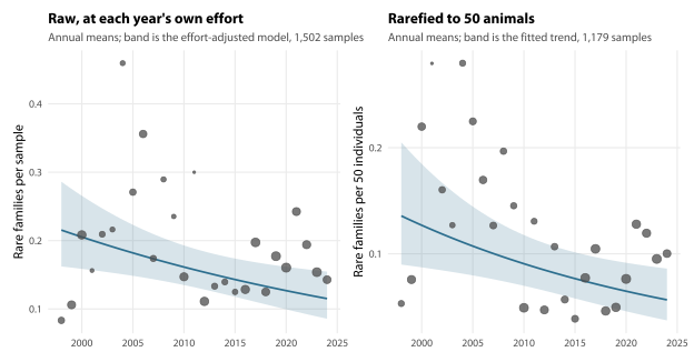
Rare families are being lost, and the effort artefact makes that finding conservative. Rare-family richness per sample falls by -21% per decade (95% CI -34% to -6.3%, n = 1,502 samples at 125 sites), and by -30% per decade on the 45 sites monitored in twelve or more years. Sensitive rare families fall fastest at -30% per decade, though with 65 occurrences in the whole record the interval is wide (-51% to +0.7%) — and Section 10.4.2 is where that particular figure gets tested and does not entirely survive.

The asymmetry is what makes this credible. Sampling effort rose over the record, and more animals counted means more rare families detected — so the effort artefact pushes towards an apparent increase, not a decrease. Without the effort term the decline reads as only -8.7% per decade; correcting for effort makes it steeper, not shallower. A negative finding that survives a bias running the other way is a finding to take seriously.

One specification difference is worth stating here rather than leaving to the code. Table 10.4 is fitted with a site random effect only; the rarefied model in Section 10.4.1 carries a year random effect as well, and argues there that a year term is not optional, because a field round shares the weather, the crew and the picking. That argument applies to this table too, and it is not applied: the effort-modelled fit is kept as it is so that it and Figure 10.4’s left panel answer the same question. Adding (1 | yearf) here moves the headline all-rare figure from -21% to -23% per decade (-37% to -4.5%, p = 0.017), which is the same finding. The row it does change is Other rare families on all sites, which goes from -18% (-33% to -0.3%, p = 0.046) to -20% (-36% to +0.8%, p = 0.059) — an interval that no longer excludes zero. That row is not a decline this chapter will defend, and it should not be quoted as one. The all-rare decline, which is the one the chapter argues from, survives either specification.

10.4.1 The decline is not an artefact of the effort adjustment

That argument still rests on a model. The effort term assumes a particular functional form for how detection rises with the number of animals counted, and if the form is wrong the trend inherits the error. Too much rests on this to leave a functional form in the middle of it, so the assumption is removed altogether and effort held constant by construction.

Rarefaction does that. For every sample containing at least n individuals, the hypergeometric expectation gives the number of rare families that would have been detected in a random subsample of exactly n animals — the same quantity for a 40-animal sample and a 400-animal one. The trend is then fitted to that, with no effort term in the model at all.

Table 10.5: Rare-family richness rarefied to a constant number of individuals per sample, fitted with no sampling-effort term (Tweedie mixed models with a site and a year random effect). Samples holding fewer than the stated number of individuals cannot be rarefied to it and drop out, which is why n falls as the rarefaction size rises. For comparison, the effort-adjusted estimate on all 1,502 samples is -21% per decade.

Response	Rarefied to	Samples	Sites	Change per decade	p
All rare families	30 individuals	1,357	125	-24% (-41% to -0.9%)	0.043
Sensitive rare families	30 individuals	1,357	125	-39% (-59% to -8.0%)	0.018
All rare families	50 individuals	1,179	118	-29% (-44% to -8.3%)	0.008
Sensitive rare families	50 individuals	1,179	118	-34% (-55% to -1.0%)	0.045
All rare families	100 individuals	732	96	-21% (-40% to +3.8%)	0.091
Sensitive rare families	100 individuals	732	96	-21% (-56% to +44%)	0.441

Held at a constant 50 animals per sample, rare-family richness falls -29% per decade (95% CI -44% to -8.3%, p = 0.008, n = 1,179 samples at 118 sites) — steeper than the -21% the effort-adjusted model gives. The decline is not manufactured by the effort correction. It is demonstrated against effort rather than adjusted for it. Rarefied to 50 individuals, mean rare families per sample runs 0.155 (1998–2004), 0.139 (2005–2011), 0.069 (2012–2018), 0.094 (2019–2025).

That is the number to quote from this chapter, and it should never be quoted without its interval: the model is a Tweedie GLMM with a log link, rare_50 ~ td + (1 | sitecode) + (1 | year). The year random effect is not optional — a field round shares the weather, the crew and the picking — and it widens the interval by about a fifth, which is the honest width.

The check is weaker at 100 individuals (-21%, p = 0.09), but only 732 of the 1,502 samples hold that many animals and those are concentrated in the later, higher-effort years, so the test loses both power and the early record at once. The sensitive rare families alone decline at every rarefaction size in Table 10.5, significantly at 30 and 50 individuals.

This chapter rarefies to 50 animals and the rating chapters rarefy to 20. That is deliberate, and Section 3.4.3.3 settles it once for the whole book — do not read a richness figure from here against one from chapter 15 without going there first.

Figure 10.4: The rare-family decline, twice. On the left, the raw annual means at each year’s own sampling effort, with the effort-adjusted model prediction at constant average effort drawn over them: the points and the line are on different footings, and the raw means do not fall, because sampling effort roughly doubled over the record. On the right, the same record with effort removed by construction — every sample rarefied to fifty individuals — where the points and the fitted trend answer the same question and both fall. The right panel is the honest picture of the decline.

10.4.2 Does the threshold decide the answer?

Everything above rests on one arbitrary number: a family is rare if it appears in fewer than 20 of the 1,502 samples. That threshold sets the 42-family set, the two-group split and the decline, so it is refitted here at 15, 20, 30 samples rather than defended.

Table 10.6: The trend in rare-family richness refitted at three definitions of ‘rare’. The middle cut, fewer than 20 samples, is the one used throughout this chapter. Raising it to 30 adds 12 families, 5 of them sensitive by this chapter’s rule (Antipodoeciidae, Calocidae, Coloburiscidae, Helicophidae, Nannochoristidae). The sensitive rows for the two lower cuts are identical because all 13 sensitive rare families appear in fewer than 15 samples, so only the cut of 30 changes that group.

Cut	Families	Group	Set	Change per decade	p
< 15 samples	38	All rare	All sites	-16% (-30% to +2.3%)	0.083
< 20 samples	42	All rare	All sites	-21% (-34% to -6.3%)	0.007
< 30 samples	54	All rare	All sites	-12% (-23% to -1.0%)	0.034
< 15 samples	38	All rare	Panel	-15% (-34% to +9.8%)	0.212
< 20 samples	42	All rare	Panel	-30% (-44% to -12%)	0.002
< 30 samples	54	All rare	Panel	-17% (-29% to -3.3%)	0.017
< 15 samples	13	Sensitive rare	All sites	-30% (-51% to +0.7%)	0.054
< 20 samples	13	Sensitive rare	All sites	-30% (-51% to +0.7%)	0.054
< 30 samples	18	Sensitive rare	All sites	+14% (-8.8% to +43%)	0.246
< 15 samples	13	Sensitive rare	Panel	-48% (-68% to -13%)	0.013
< 20 samples	13	Sensitive rare	Panel	-48% (-68% to -13%)	0.013
< 30 samples	18	Sensitive rare	Panel	+13% (-15% to +51%)	0.390

The all-rare decline is not an artefact of where the threshold was put. The sensitive-family decline partly is. The whole rare set falls at all three cuts, at between -12% and -21% per decade across all sites — significantly at cuts of 20 and 30, and short of it at 15 (p = 0.08), where the set is smallest and the counts sparsest. The sensitive subgroup runs at -48% per decade on the panel at the threshold used here, and at a cut of 30 it does not fall at all (+13%, p = 0.39).

The reason goes here rather than in a footnote, because it is the one attack on the rare-family finding this chapter cannot close. The 5 sensitive families a cut of 30 adds, named in Table 10.6’s caption, are recorded 21–26 times each and are heavily concentrated in the later record: Antipodoeciidae, for instance, has 24 of its 26 records after 2011 and none before 2006. That is what a family entering the laboratory’s working list part-way through the record looks like, as much as it is a family becoming commoner. Until we can see the laboratory’s taxonomic reference list by year, a decline in a moderately common sensitive family cannot be separated from a change in whether it was being distinguished — which is why dq:dated-family-list is the most valuable single item this chapter puts on your list.

So: argue the conservation case from the whole rare set, which declines at every threshold tested and declines under rarefaction, which no change in identification practice would produce. Quote the sensitive-family rate only with this paragraph attached to it.

10.4.3 What has already gone

12 of the 42 rare families have not been recorded since 2009 or earlier, 4 of them sensitive: Eustheniidae (last 2001), Oeconesidae (last 2004), Eusiridae (last 2006), Osmylidae (last 2009). Most were recorded once or twice to begin with, so absence is weak evidence of loss for any individual family.

Three of the 12 should be discounted before the pattern is claimed, and the deduction is worth showing rather than asserting. Spercheidae and Gomphomacromiidae are two of the six taxon names the data layer reports as unmatched to the taxonomy after normalisation, and Gomphomacromiidae is in any case a name since absorbed into other dragonfly families — its disappearance in 2006 is a nomenclature event, not an extinction. Eusiridae’s single 2006 record is very likely the same animal that appears from 2010 as Paramelitidae, the family Australian freshwater eusirids were transferred to. That leaves 9.

Nine simultaneous disappearances in a record whose sampling effort was rising is a pattern, not a coincidence — and here is the test. Allocating each rare family’s observed number of occurrences at random across the samples, with probability proportional to the sample’s abundance raised to the fitted detection exponent so that the rising effort sits inside the null, 2,000 replicates expect 3.8 families to fall silent by 2010 and put the upper end of the 95% range at 7. The observed 9 gives P = 0.004.

The sensitive families are a separate claim, and it is the deduction that decides it. Four of the original 12 were sensitive, and against that 4 — which is above the 1.7 chance expects — the randomisation returns P = 0.039. But Eusiridae is one of the 4, and one of the three struck out. Of the 9 that survive the deduction, three are sensitive: Eustheniidae, Oeconesidae, Osmylidae. Run against three, on the same 2,000 replicates and the same null — which still allows any of the 13 sensitive rare families to fall silent, so the deduction can only make the test harder to pass — the observed 3 gives P = 0.205. So the sensitive half of this result does not stand on the deducted set the way the overall half does, and it must not be quoted as though it did: on the 9 this chapter is prepared to defend, the sensitive families are not distinguishable from chance.

Eustheniidae (a large stonefly), one of the most sensitive animals in the Australian fauna, was last recorded in 2001.

10.5 Where what is left is concentrated

Among the 95 sites with at least five samples, the number of sensitive rare families recorded is 2 sites with 3, 8 sites with 2, 29 sites with 1, 56 sites with 0. Exactly 10 sites have recorded more than one. Table 10.7 is the list; everything below them is a tie.

Table 10.7: The 10 sites recording more than one sensitive rare family, among the 95 sites with at least five samples. ‘n’ is samples; ‘Alt m’ altitude; ‘Tier’ catchment disturbance tier; ‘Imp %’ total catchment imperviousness; ‘Fines’ and ‘Shade’ the site-mean percentage of silt-and-clay substrate and of canopy shading; ‘Sens.’ the number of sensitive rare families recorded; ‘Restr.’ the number of rare families found at five sites or fewer anywhere in the record; ‘Boot.’ the proportion of 1,000 bootstrap resamples in which the site is among the twelve highest counts, with ties broken at random. A dash means the value is not recorded for that site — no delineated catchment, no site description, or no recorded altitude.

Creek (site)	n	Alt m	Tier	Imp %	Fines	Shade	Sens.	Restr.	Boot.
Pierces Pass Creek (60GBLR)	14	740	Ref	0.6	0.8	95.3	3	1	0.91
Pulpit Hill Creek (10BMG)	21	686	Slight	2.8	3.6	52.8	3	2	0.79
Glenbrook Creek (51NGK)	18	64	Slight	1.9	2.4	20.7	2	2	0.67
Bedford Tributary (P2-M5)	7	–	Urban	11.0	–	–	2	1	0.63
Lillians Glen (22.2BWF)	10	782	Slight	14.7	1.8	70.9	2	1	0.65
Wentworth Creek (25.2GWF)	8	750	Slight	5.2	3.8	68.6	2	0	0.54
Cedar Creek (54BMGR)	13	150	Ref	0.0	2.6	64.2	2	1	0.54
Hat Hill Creek (06GBH)	24	962	Slight	9.6	5.0	49.3	2	0	0.54
Terrace Falls Creek (31EHZ)	24	574	Slight	7.4	4.4	46.1	2	0	0.57
Knapsack Creek (50NEP)	23	52	Urban	18.2	3.9	43.1	2	3	0.64

These are the creeks worth protecting, and there are ten of them. Pierces Pass Creek (60GBLR) heads the list: a reference creek with 3 sensitive rare families, 0.8% fine sediment and 95.3% canopy shading. Pulpit Hill Creek (10BMG) and Glenbrook Creek (51NGK) follow.

Eight of the ten are urban or slightly disturbed creeks, not reference sites. That is the whole point. Reference creeks are protected by being remote. These are creeks with something unusual in them sitting in catchments you manage, and several of them are not in good condition by the current rating. A condition rating will never flag them, because condition is not what makes them valuable.

A longer list than this cannot be defended, so here is where it stops and why. 29 of the remaining sites have recorded exactly one sensitive rare family and cannot be separated from one another on this record. Extending the list to twelve means breaking that tie, and the two sites it would add — Bedford Creek (30EHZ) and Kedumba Creek (85BKT) — have no better claim than several that would still be left out. Resampling the samples within each site 1,000 times and re-ranking with ties broken at random, the 10 named sites appear in a top twelve with probability 0.54 to 0.91, while those two appear with probability 0.27 and 0.20 — and 5 other creeks, none of them named, appear at least as often. 39 distinct sites enter the top twelve in at least one resample. Any list longer than ten is reporting a tiebreak as a rank. If you want a twelve-site program, choose the last two places on a stated criterion — restricted-family count, catchment spread, tenure — and not on a tiebreak nobody sees.

10.5.1 One family deserves naming on its own

Paramelitidae (a freshwater amphipod) is the most concentrated rare family in the analysis set: 6 records over just 2 sites, the highest ratio of records to sites of any of the 42 in Table 10.2. Counted over the whole archive — which for this one question means including the riffle samples the rest of the chapter excludes, because where an animal has been found is a conservation claim rather than an analysis result — there are 7 records at 3 sites and 178 individuals, set out site by site in Table 10.8.

Table 10.8: Every record of Paramelitidae in the archive (7 records, 178 individuals). The Blue Gum Swamp Creek record is a riffle sample and is therefore absent from every other analysis in this chapter.

Creek (site)	Records	Individuals	Years
Waterfall Creek (01CMW)	5	172	2010–2024
Blue Gum Swamp Creek (41NWL)	1	3	2006
Knapsack Creek (50NEP)	1	3	2021

This is one established population and two isolated detections, not two or three populations. 5 of the 7 records and 172 of the 178 individuals are from Waterfall Creek (01CMW), where the family has been found in five years — 2010, 2015, 2016, 2020 and 2024 — in counts of 100, 4, 29, 3 and 36. 14 years of repeated detection in numbers at one reach is the signature of an established local population rather than a stray. The other two records are three animals each, once, at Blue Gum Swamp Creek (41NWL, 2006) and Knapsack Creek (50NEP, 2021). Each of those, on its own, is as consistent with a stray as with a population.

The average of 25 animals per record is carried by the single 2010 sample of 100; the median record is 4.0 animals. That matters more than a family record usually would. Australia’s crangonyctoid amphipods, of which Paramelitidae is one of three families, are the dominant amphipods of cold running fresh water here and are strongly regionally differentiated, with many species known from very few localities (Williams and Barnard 1988); short-range endemism — Harvey’s criterion is a natural range under 10,000 km², and many Australian crangonyctoid amphipods are known from a handful of localities within one (Williams and Barnard 1988) — is the reason a single well-established population can carry conservation significance that no condition rating will ever register (Harvey 2002).

Nothing here can identify the animal to species. That needs a specialist, and the specialist should be sent to Waterfall Creek, where there is a population to identify. The other two creeks warrant a confirmatory survey to establish whether there is anything there at all — not a specialist identification of a population that has not yet been shown to exist.

10.6 What we think you should do about it

Create a protection tier, separate from the condition rating.

1. Flag, do not score. Adding a rare-family bonus to the rating would change about 1% of ratings, because 96% of samples contain no sensitive rare family at all. A flag on the site record is the right instrument; a score component is not.
2. List the ten sites in Section 10.5 as high conservation value, review the list annually against new records, and attach the flag to the site rather than to the sample. Do not extend the list without new records to justify it: below that point the sites are tied and the ranking is arbitrary.
3. Commission a specialist identification of the Paramelitidae population at Waterfall Creek (01CMW), which is where the population is. If it is a short-range endemic, that single fact changes how that catchment should be managed. Re-survey Blue Gum Swamp Creek and Knapsack Creek for the same animal at the same time; a single detection at each is worth checking and is not yet a second population.
4. Protect what the sensitive rare families need. Of the 18 site variables tested, false-discovery control leaves one — catchment area. Fine sediment on the bed and dissolved oxygen point the same way without clearing the correction, and sediment control during works — in these ten catchments in particular — is the most direct lever available on any of them.
5. Report the protection tier beside the condition rating, not inside it.

The cost is close to zero. The consequence is that you can see, and act on, the one thing in your own dataset that is measurably and quietly going.

One caveat belongs on the file with this, and it is the one from Section 10.4.2. The case above rests on the rare families as a whole — the group that declines at every threshold tested and declines again when effort is removed by rarefaction. It does not rest on the -48% figure for the sensitive subgroup, which reverses at a cut of 30 samples. If someone attacks this recommendation, that is where they will attack it, and the answer is that the recommendation never needed that number.

And the thing that would most improve all of it: dq:dated-family-list. A dated version of the laboratory’s family reference list closes the last open attack on the most consequential conservation claim in this report, and it is a filing-cabinet search rather than new fieldwork.

Benjamini, Yoav, and Yosef Hochberg. 1995. “Controlling the False Discovery Rate: A Practical and Powerful Approach to Multiple Testing.” Journal of the Royal Statistical Society, Series B 57 (1): 289–300. https://doi.org/10.1111/j.2517-6161.1995.tb02031.x.

Harvey, Mark S. 2002. “Short-Range Endemism Amongst the Australian Fauna: Some Examples from Non-Marine Environments.” Invertebrate Systematics 16 (4): 555–70. https://doi.org/10.1071/IS02009.

Jones, J. I., J. F. Murphy, A. L. Collins, D. A. Sear, P. S. Naden, and P. D. Armitage. 2012. “The Impact of Fine Sediment on Macroinvertebrates.” River Research and Applications 28 (8): 1055–71. https://doi.org/10.1002/rra.1516.

Williams, W. D., and J. Laurens Barnard. 1988. “The Taxonomy of Crangonyctoid Amphipoda (Crustacea) from Australian Fresh Waters: Foundation Studies.” Records of the Australian Museum, Supplement 10: 1–180. https://doi.org/10.3853/j.0812-7387.10.1988.94.

Wood, Paul J., and Patrick D. Armitage. 1997. “Biological Effects of Fine Sediment in the Lotic Environment.” Environmental Management 21 (2): 203–17. https://doi.org/10.1007/s002679900019.