3  How the method changed, and what it cost

Blue Mountains City Council Healthy Waterways — statistical analysis

3.1 What this chapter is for

A monitoring record holds two things at once: what the creeks did, and what the program did. Over 27 years this program changed the number of animals its laboratory picked out of a sample, what it asked to have identified, which habitat it sampled, what month it went out in, and which probe it carried — and, somewhere in the nine-month sampling gap between 6 May 2004 and 1 February 2005, something at the bench moved every faecal coliform count by about a hundredfold. None of those changes was written down as a change. Every one of them leaves a mark that looks exactly like a creek getting better or worse.

That is what this chapter is about, and the short version is this: a large part of what looks like change in this record is change in how the record was made.

Each of these was found by a different analysis tripping over it, and until now each was re-explained in whichever chapter hit it first. Gathering them here is not tidiness. It is the only way to see that they are one problem — the program was never asked to hold its method constant, because nobody was ever going to read it as a time series — and that most of them have the same fix, which is a fortnight of somebody’s time and a filing cabinet.

One piece of bookkeeping before Table 3.1, because it recurs. The two databases do not cover the same period. The macroinvertebrate record runs October 1998 to August 2024, about 26 years; the water quality record runs January 1998 to June 2025, about 27. So a statement about richness or rarefaction spans 26 years and a statement about a probe or the program as a whole spans 27, and neither figure is the right one for the other. Both are correct and they are not interchangeable.

Two things this chapter is not. It is not a case that the monitoring was done badly: every one of these changes is a normal thing for a long-running program to do, and several of them were improvements to the measurement at the moment they were made. And it is not a case that the record cannot be used. Most of it can. What the chapter does is say, for each measure, how much of its apparent movement is method, whether that part can be separated out, and what it would take to separate it.

3.2 The verdict table

One row per method change. What it affects names the measures that carry the change into a published number; separable? says whether the effect of the method can be taken out of the data we have, or whether it can only be worked around by narrowing the question.

Table 3.1: Every method change this report has had to work around, what it moves, and whether it can be separated from the environment. Sizes are as derived in the sections named; the macroinvertebrate figures are over 1,503 edge stream samples from 125 sites and the water quality figures over 1,304 stream samples.

Method change	When	How big	What it affects	Separable?
Animals picked per sample rose (Section 3.4)	gradual, sharpest 2008-2011	median 92 to 167 individuals; 1.39x per decade within site	family richness, EPT richness, %EPT, the health score	Partly. Rarefaction removes it, at the cost of 22% of samples
Chironomid identification changed twice (Section 3.5)	2000-01 family-only; 2008-09	recorded in 0% of 43 samples in 2008 and 14% of 36 in 2009; 8-21% of individuals in a normal year	the published family count, %EPT, SIGNAL-SF	Yes. Use n_families_strict, or a chironomid-free check
Riffle sampling ceased (Section 3.6.1)	after 2007	riffle scores +0.26 above the paired edge sample; all 338 riffle samples affected	the health score and its rating, 1998-2007	Yes. Filter on band_applicable, or show edge-only
The sampling calendar drifted (Section 3.7.1)	across the record	median sampling date 2 March to 26 May, about 3 months	every temperature-sensitive water quality parameter	Yes. Two day-of-year harmonics
The probe was replaced twice (Section 3.7.2)	2017 and 2020	turbidity site median 4.73 to 0.058 NTU, falling at 54 of 55 sites; dissolved oxygen +0.79 then +0.66 mg/L	turbidity, dissolved oxygen, conductivity, salinity	No. There is no overlap period at either changeover
Detection floors substituted (Section 3.7.5)	throughout	one of seven floors is a confirmed measurement limit and four are substitution points chosen here; the trend estimate moves tens of percentage points across defensible choices	phosphate, nitrate-N, turbidity, faecal coliforms	Partly. Report exceedance rather than level
Something changed at the bench (Section 3.7.6)	6 May 2004 to 1 February 2005	a fall of 1.90 log10 (1.69 to 2.11), about 79-fold, the same at all 33 paired sites	the whole faecal coliform record before 2005	No. Analyse from 2006 and lose seven years
Habitat recorded by eye, and drifting (Section 3.6.2)	2008 on	10 of 13 variables drift at a site that did not move; riparian shading +11.7 points per decade	the physical habitat block, and the shading recommendation	Partly. Aerial imagery settles shading (Section 3.6.3)

Read down the last column of Table 3.1 and the chapter’s practical message is there. Six of the eight can be worked around: rarefy the counts, use the strict family list, filter to edge samples, put day-of-year in the model, report exceedance instead of concentration, settle the shading from aerial imagery. Two cannot be worked around at all — the probe replacements and the bench change — and a third, the animals picked per sample, can be worked around only by throwing samples away. The reason is the same in all three cases — nothing was measured twice. No sample was picked to two different target counts, no site was read by both probes on the same day, no split sample was sent to the laboratory either side of the 2004 change. A confound you have measured twice is arithmetic. A confound you have measured once is permanent.

That is the recommendation this chapter really makes, and it is cheap: whenever the method changes, run the old and the new alongside each other for one round. Section 3.8 says what that costs and what it is worth.

3.3 The data behind this chapter

Each question and request below is set out again in What we need from you, with what it blocks, what an answer is worth and what it would cost you to find, ranked against every other ask in the report.

3.3.1 What this chapter uses, and where it came from

Every method change in this chapter was inferred from the pattern in the numbers. Not one of them was found written down.

Neither database records a pick count, a subsampling protocol, a laboratory method, a test-kit change, a datasheet revision or a field officer before 2018. So the eight changes in the verdict table (Table 3.1) are read off the data: a step that happens at every site on the same date, a count that doubles, a group of animals that vanishes for a year, a column that appears in 2008 and none before. The inferences are strong — a hundredfold improvement in undeveloped bushland on the same day as everywhere else is not an environmental result — but every one of them could be settled or overturned by a single piece of paper, which is why the asks below are worth more than any further analysis.

Blocks: Nothing on its own; it is why the rest of this list exists. Value: high. Costs you: minutes. Refer to it as dq:method-changes-inferred-not-documented.

The aerial canopy test uses your Nearmap historical archive — 17 captures over 2014 to 2021, classified in a 30 m buffer at 123 located sites.

Rebuilding it needs your Nearmap key and about 8,000 licensed tiles, so the comparison is kept as a tracked derived file rather than recomputed. Every capture was flown between July and October, so sun angle and phenology are about as constant as the archive allows. The archive is not calibrated between captures, which is why the test can compare a site with itself across years but cannot say what canopy did across the network.

Blocks: Nothing — this is a statement of what we used. Value: low. Costs you: minutes. Refer to it as dq:canopy-archive-provenance.

The two numbers this chapter publishes to the rest of the report are fitted once in the pre-render harness, not in the chapter.

Rarefied richness (Hurlbert expectation on the strict, microfauna-free edge matrix at depths 20, 30, 50 and 100) is read by three chapters and the summary, and the %EPT effort attenuation by two. Both are fitted in data-layer/prerender.R and read here like everywhere else, and every reading chapter asserts that its own analysis set matches the one the fit used. Chapters 8, 10 and 15 rarefy different things and quote the result rather than the series; that is deliberate and should not be unified.

Blocks: Nothing — this is a statement of how the numbers travel. Value: low. Costs you: minutes. Refer to it as dq:rarefaction-and-ept-fitted-once.

3.3.2 What is wrong with it

No sample was ever measured both ways — not at either probe change, not at the 2004 laboratory change, and not at any change in the pick count.

This is the single structural reason three of the eight method changes cannot be corrected. Over a six-year window a step and a trend are nearly the same regressor, so the tests can show that something changed at a boundary far better than they can show how much: only 7 of the 44 estimated shifts survive giving each year its own level, and none of the dissolved oxygen or conductivity ones do. Two field rounds with both instruments in the car would have replaced every one of those sentences with a correction factor. The next replacement is the opportunity, and it will be missed by default unless the overlap is written into the procurement.

Blocks: Any turbidity, dissolved oxygen or coliform series spanning a changeover; the size, as opposed to the existence, of every instrument step. Value: transformative. Costs you: minutes. Refer to it as dq:no-overlap-at-any-changeover.

The 2004-05 coliform break falls inside a nine-month hole in the sampling, 6 May 2004 to 1 February 2005, and no test can place a step inside a window with no data in it.

Profiling the break over candidate dates returns an interval that is not really a statistical result — it is the shape of the gap. 2005 is already on the far side of it: of that year’s readings, all but two are at post-break levels, and the two exceptions are a single day in April. So neither “the series breaks in 2005” nor “the series starts in 2006” says anything about when the measurement changed. 2006 is an analysis choice, not a break date.

Blocks: Joining the coliform record into one series; four years of coliform data, 2002 to 2005. Value: high. Costs you: minutes. Refer to it as dq:coliform-break-undatable.

The field officer is recorded on only 227 of the stream site descriptions, all of them between 2018 and 2024, and each officer works a block of months — so observer and period cannot be separated on this record.

Five officers is five observations of an officer effect however many descriptions they wrote between them, which is why every variance share in the chapter carries a bootstrap interval and why the intervals are enormous. Give the year its own term and most of the officer signal transfers to it. Aerial imagery breaks the confounding for riparian shading, because it is independent of every officer; nothing breaks it for moss, detritus or macrophyte cover.

Blocks: Modelling the observer rather than ruling them out; the reading of the habitat block in chapter 9. Value: high. Costs you: minutes. Refer to it as dq:officer-and-period-confounded.

Standardising the counts by rarefaction discards 21.6% of samples at the research depth of 50, and they are not a random fifth — they are the early, low-scoring ones.

That is what makes the working-around expensive rather than free. Three checks say the flat rarefied series is not an artefact of the discarding — the answer is the same at every depth from 20 to 100, an effort control that discards nothing agrees, and the discarded samples are improving too — but all three would be unnecessary if the pick count had been fixed, or simply recorded. At the rating depth of 20 the loss is 71 samples rather than 324, which is why the report uses two depths.

Blocks: Nothing on its own; it is the cost of the workaround, and a large part of why the pick-count question is among the most valuable asks on this list. Value: moderate. Costs you: minutes. Refer to it as dq:rarefaction-discards-early-samples.

3.3.3 Questions only you can answer

Did two probes ever go out on the same site on the same day — even a handful of samples, even informally during a changeover?

Turbidity fell about eightyfold across the two instrument changes, at 54 of the 55 stream sites measured both before and after: the site median goes from 4.73 NTU over 2012-16 to 0.058 NTU over 2020-24. Creeks do not do that; sensors do. Dissolved oxygen steps up 0.79 mg/L at the first change and 0.66 at the second, which is more than its whole apparent improvement over the record. With even a few days where both instruments were used we can stitch the three eras into one 27-year record. Without it, turbidity and dissolved oxygen have simply been abandoned. It is a yes/no question and the answer is worth two whole parameters.

Refer to it as dq:side-by-side-runs.

When the lab wrote a plain 0 for phosphate, nitrate-N or faecal coliforms, did it mean “none detected” or “below what the test can see”? And is the 5 written for coliforms from 2020 the same thing?

More than half the phosphate readings in twenty-three years — 53.8% — sit below what the method could see, nearly all of them written down as an exact zero, and a third of the coliform ones. If they mean “below the detection limit”, then the cheerful finding that phosphate improved is mostly a story about test kits, and a published range starting at 0.00 has been silently scoring every non-detect as a pass. If they are real zeros, the finding stands. One person who worked the bench can answer this in a sentence, and nothing else on this list has that ratio.

Refer to it as dq:zeros-are-nondetects.

On the 160 visits with more than one macroinvertebrate sample, why was the second one taken — a separate collection from the creek, one collection split in two, or the lab checking itself? Registration books or lab submission forms would show it.

The most quoted number in the whole report is that two samples from the same creek on the same day land in different published rating classes 38% of the time, over the 144 two-sample visits — an observed count, rising to 41% of all 160 visits if the 16 with three or more samples are included. That 41% is not the modelled 41% the executive summary quotes for a three-year rating; the two are unrelated quantities that happen to round to the same two digits. What this one means depends entirely on which of those three it is. If they are split subsamples, 38% is a lower bound. If they are lab duplicates, the fix is laboratory QC, not more field visits. You are being asked to spend money on the strength of a number whose meaning is currently unknown, and this decides which budget line it comes out of.

Refer to it as dq:replicate-purpose.

Chironomids vanish from the records in 2008 and appear in only 5 of 36 samples in 2009. Was that a lost data-entry batch, or did somebody change what the lab was asked to identify?

Chironomids average 14% of the individuals in a sample and one to three rows of the family count, so both the family count and %EPT are distorted across those years. The choice is between excluding two years and modelling the change, and we cannot make it without knowing which happened. Somebody may simply remember.

Refer to it as dq:chironomid-absence-2008.

On the Hydrolab and Aquaread, was salinity in PSU computed from electrical conductivity by a fixed factor — and if so, which factor?

Pre-2020 salinity is recorded on a 0.01 PSU grid, and the published desirable range is exactly one quantisation step wide, so no pre-2020 salinity rate or trend means anything at the moment. If PSU was derived from EC by a known factor we can reconstruct it at full precision from the EC column and get the whole parameter back. One number does it.

Refer to it as dq:salinity-psu-derivation.

The Macro round has drifted from early March to late May over the record. Can it be pinned to a fixed window from now on — and does anything (staff, budget cycle, weather, contractor availability) make one window easier to hold than another?

The median sampling date moved from 2 March over 1998-2005 to 26 May over 2020-2025, about three months, out of late summer and into late autumn. That is the largest single confound in the water quality record and it is almost entirely correctable in analysis — every model in the report carries two day-of-year harmonics — but it is much better fixed at the source. What it does when it is not corrected: water temperature appears to be falling by 1.8 °C per decade, and the same data with the seasonal terms in say it is rising by 0.6 (95% CI 0.31 to 0.85, 1,290 samples). Not a smaller trend, the opposite sign. This is the one item on the list that costs nothing to answer and needs a decision rather than a document: pick a four-week window and hold it.

Refer to it as dq:sampling-calendar-drift.

Which physical instrument do the four device labels and two serial numbers in the database correspond to — and what was used on the 135 Aqua TROLL-era turbidity readings that carry no device identifier?

Housekeeping, but it is what lets an instrument step be pinned to an instrument rather than to a date. Somebody who was there will know this straight away.

Refer to it as dq:probe-device-labels.

3.3.4 What would answer them

How many animals was the laboratory asked to pick out of each sample, was any subsampling used, and on what dates did either change? Even a dated instruction or an email thread would settle it.

The median number of animals found per edge stream sample went from 92 over 1998-2009 to 167 from 2014 on, a factor of 1.39 per decade within a site. That is either creeks getting healthier or somebody picking harder, and nothing in the archive distinguishes them. Adjusting for it removes about a third of the headline improvement in waterway health — the single most important number in the report. An entire chapter’s worth of statistical machinery exists to work around this one missing document, and it throws away a fifth of the samples doing it. If the answer is “there was no protocol”, that is still the answer, and it says start recording it today.

Refer to it as dq:pick-count-protocol.

Which test kit or method did you use for phosphate and nitrate-N, and what does its packaging or instruction sheet say it can detect? A purchase order, a stores ledger entry or a photograph of a kit box would all do it.

We have had to guess at this, and the guess was wrong once already, which is why it is near the top of the list. Nothing in either database records what the method could detect — so the limit was taken from the smallest value the data held, 0.005 ppm, and that value turned out to be one our own arithmetic produced. Seven phosphate and three nitrate samples between 22 February and 27 April 2012 are each the average of a laboratory duplicate reading 0.00 and 0.01. The raw table holds nothing below 0.010 in any year and every reading sits on a 0.01 grid, so we now use 0.010 — and making that correction moved those ten samples from “measured” to “not detected”. A number that decides whether a reading is a measurement or an absence should not be coming out of our averaging. Two things suggest where to look. tblSamples.LabOfficer names Council staff rather than a laboratory, and the coliform notes describe 1 mL and 10 mL aliquots plated in-house — so this looks like a bench or field test kit, and a 0.01 ppm grid unbroken across twenty-two years is what a colorimetric kit produces. A commercial laboratory would report continuous values against a stated limit of reporting, which is exactly the document we are missing. And the grid only tells us the resolution the results were written at, not the floor of the kit that produced them: the only two field notes that state a floor disagree, “Phos <0.1, Nitrate <0.1” in September 2008 and “Phos<0.01, Nitrate <0.01” five months later, both recorded beside a stored zero. If the kit or its range changed between those two dates, that would be worth knowing too. Coliforms are separately documented at 10 CFU/100 mL in the field notes and need no further work. The same kit box would settle one more thing, asked separately as dq:phosphate-units: whether the phosphate result is written as PO₄ or as P. Nothing in either database, the field sheets or the methods document says which, the two differ by a factor of three, and every phosphate concentration in ppm in this report is ambiguous by that factor until it is answered. Your nitrogen field says which it is — it is called Nitrate-Nitrogen — and the phosphate field does not.

Refer to it as dq:lab-detection-limits.

Was there ever a training note, induction, worked example or run sheet on how to estimate cover — anywhere between about 2010 and 2016? A dated version of the site description form would also do it.

Recorded riparian shading rises 11.7 percentage points a decade at sites that have not changed, while moss, detritus and trailing vegetation drift down. Aerial imagery has now shown officers are right about which reaches are shady and that their year-to-year movements at a fixed reach do not track canopy — so the rise is in the recording, not the trees. What imagery cannot recover, at any budget, is why. A training record from the mid-2010s would. This matters because the report’s main practical suggestion is “shade your creeks”, and it rests on that variable.

Refer to it as dq:training-record-2010-2016.

Do you have the manufacturer’s turbidity sensor specification and stated resolution for the Hydrolab Quanta, the Aquaread AP-2000 and the In-Situ Aqua TROLL 500? A data sheet or a manual would do.

We have had to invent a 0.1 NTU detection floor with no documentary basis whatsoever, and three headline percentages in the water quality chapter rest on it. A published spec sheet replaces our invention with a fact.

Refer to it as dq:probe-specs.

Did the nutrient test kits change over 2017-2019? Anything at all — a supplier change, a new reagent, a different reading method?

The share of phosphate results below the detection limit runs 75-89% over 2013-2016, falls to 17-34% over 2017-2019, and returns to 61-90% from 2020. Creeks do not do that. Something in the method is switching back and forth, and until we know what, none of those years can be read as a nutrient signal.

Refer to it as dq:nutrient-2017-2019-change.

Something changed at the bench over the summer of 2004-05 and faecal coliform counts fell about a hundredfold. Is there a method log, an SOP from 2003-2006, an analysis report or an invoice that would say what?

The step is identical at every site, including the unsewered reference catchments, which rules out sewer works and points squarely at the laboratory. Field sheets for the summers of 2004 and 2005 would help too. As it stands, twenty-four years of coliform data cannot be joined into one series across the break.

Refer to it as dq:coliform-2004-break.

Who did the field work, and on which dates, back to 2006? Field diaries, run sheets, timesheets or payroll would all work.

Before 2018 the officer and the period are completely confounded, so we can rule the observer out but never model them. Field officer takes 22-24% of the variance in algal and macrophyte cover — as much as the site itself. A roster turns that from a caveat into a term in the model.

Refer to it as dq:field-officer-roster-pre2018.

Are the laboratory identification sheets, or a LabIDOfficer roster, still around for 2000-01 and 2008-09?

This is the documentary version of the chironomid question. The bug database only records a lab ID officer from 2019 onwards, so for the two suspicious periods there is no record of who identified what or to what level.

Refer to it as dq:lab-id-roster-2000s.

Are there calibration records for the probes — particularly for the two Aqua TROLL units? They may well be on paper.

The two Aqua TROLLs disagree by 40 percentage points on how often they return a sub-floor turbidity value. Without logs that cannot be attributed to either instrument, and it narrows rather than closes the turbidity problem even if we get them.

Refer to it as dq:probe-calibration-logs.

Do the pre-2012 field sheets carry a time of day? The water quality database records a sampling time from 2012 onwards but not before.

Diurnal water temperature variation in a shaded headwater stream is 2-5 °C, and the one water quality trend that survives everything else is about half a degree Celsius per decade averaged over the year. If the hour of sampling drifted over the record it would confound that trend, and at the moment nobody can check the first fourteen years. Only worth the search if the trend gets contested.

Refer to it as dq:sample-time-recover-pre2017.

(Greater Sydney Landcare Network, not you) Streamwatch’s published 1990-2020 spreadsheet already covers Blue Mountains creeks; does GSLN hold the site-level detail and the post-2020 rounds that would sit either side of the 2005 and 2017-2019 discontinuities?

The 1990-2020 spreadsheet is on NSW SEED under CC BY 4.0 and we should fetch that ourselves rather than ask for it; what is worth asking for is what the spreadsheet does not carry. It is the only external record that might independently show whether those two breaks are in the creeks or in the method – your own records cannot explain either.

Refer to it as dq:streamwatch-records.

3.4 The laboratory is counting twice as many animals

Nobody asked for this section. It came out of the analysis, and it changes how the answer to your first question – has waterway health changed? – should be read, so it comes before the components.

3.4.1 The number of animals in a sample has roughly doubled

Figure 3.1: Total number of individuals recorded per sample, on a logarithmic scale, with a smooth adjusted for site and for field round. The median sample held 92 animals over 1998-2009 and 167 from 2014 onward. This is a change in what the laboratory processed, not necessarily a change in what was in the creek, and it inflates any metric that counts taxa.

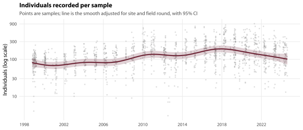
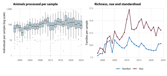
The median stream edge sample held 92 individuals over 1998–2009 and 167 from 2014 onward. Within sites, sample abundance rises by a factor of 1.39 per decade (95% CI 1.22 to 1.59), and the rise is concentrated in 2008–2011 — the same window in which the health score rose fastest.

Two explanations compete. Streams may genuinely hold more animals now; or the laboratory may be picking and counting more of each sample than it used to. Neither database records a subsampling protocol or a target pick count, so this cannot be settled from the data. What can be shown is how much it matters.

3.4.2 Number of families depends directly on how many animals you count

Family richness and sample abundance are strongly related: across the 1,503 samples the correlation between the number of families recorded and the log of the number of individuals is 0.71, and each e-fold increase in individuals is associated with 4.80 more families. That is not an ecological result, it is a sampling result — the more animals you look at, the more families you find. It applies to the number of EPT families for the same reason.

This is the best-documented artefact in rapid bioassessment and it is not a subtle one. Vinson and Hawkins (1996) showed that taxon richness rises steadily with the area sampled and the number of individuals sorted, so richness comparisons between samples processed to different effort measure the laboratory rather than the stream; Doberstein et al. (2000) found that the fixed count chosen — they tested 100 up to 1,000 individuals against fully counted samples — changed both the richness recorded and the biological verdict drawn from it, and that at counts of 100–300 the index could distinguish only about 2.8 stream classes against 8.2 for a full count, which is the band Council’s own protocol sits in; and Cao et al. (2003) give a way to measure and control assemblage data quality directly, treating sub-sampling procedure as one of the error sources it has to absorb. The Australian version of this problem was measured directly by Growns et al. (1997), who compared six sample-processing methods on the same material and found the richness recorded to depend heavily on which was used. What is unusual here is not that the effect exists but that this record contains an uncontrolled change in effort part-way through, which turns a known bias into a spurious trend.

3.4.3 Standardising the effort by rarefaction

The standard remedy is rarefaction: computing how many families a sample would have contained if a fixed number of individuals had been counted. The quantity computed is the hypergeometric expectation of Hurlbert (1971) — the expected number of families in a random subsample of n individuals drawn without replacement — which is the standard way of putting samples of unequal size on a comparable footing. Its assumptions and its limits are set out by Gotelli and Colwell (2001): it standardises for the number of individuals counted, not for how those individuals were collected, and it can only interpolate downwards, so the depth is set by the smallest sample retained.

Table 3.2: Trends in family richness before and after standardising for the number of individuals counted. Rarefied measures are the expected number of families in a random subsample of 50 individuals. Restricted to the 1,179 stream edge samples deep enough to rarefy to 50.

Measure	Period	Samples	Change per decade	95% CI
EPT families per 50 individuals	1998-2024	1,179	0.58	0.36 to 0.79
EPT families per 50 individuals	2010-2024	790	0.13	-0.41 to 0.66
EPT families recorded	1998-2024	1,179	0.96	0.67 to 1.24
EPT families recorded	2010-2024	790	0.07	-0.57 to 0.71
Families per 50 individuals	1998-2024	1,179	0.05	-0.39 to 0.50
Families per 50 individuals	2010-2024	790	-0.85	-1.65 to -0.05
Families recorded	1998-2024	1,179	1.91	0.95 to 2.87
Families recorded	2010-2024	790	-1.49	-2.76 to -0.22

Every sample with at least 50 individuals in the strict, microfauna-free community matrix is rarefied to 50. That retains 1,179 of the 1,503 samples in the primary set, or 78%. The threshold bites harder than the raw abundance column suggests — 89% of samples record at least 50 individuals in total_count, but the matrix used for rarefaction drops microfauna and lumps relabelled sub-family rows, so the median sample’s matrix total is about 17% below its total_count. That is a median and not a rate every sample pays: shrinking every sample by it would still leave 85% of them above the line. Retention falls to 78% instead because the loss is uneven — the 163 samples the threshold drops are ones losing about 47% each.

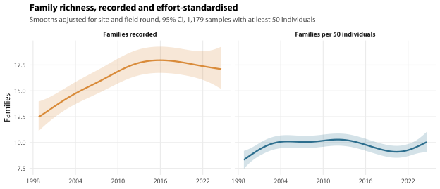
The number of families recorded has risen; effort-standardised richness has not — and the flat whole-record figure is the average of a rise and a fall, not the absence of both. Raw family counts rise by 1.91 families per decade (0.95 to 2.87). Standardised to a fixed count of 50 individuals and a strict family list, the whole-record trend is 0.05 families per decade (-0.39 to 0.50) — no net change over the 26 years.

But standardised richness has been falling for a decade. Over 2010–2024 the same measure falls -0.85 families per decade (-1.65 to -0.05), an interval that excludes zero, and the raw count falls with it (-1.49, -2.76 to -0.22) — so this is a decline in the creeks and not an artefact of standardising. Both rows are in Table 3.2 above. The smooth in Figure 3.2 has the same shape: it climbs from about 8.3 families per 50 individuals at the start of the record to about 10.1 by 2005, holds near that level to about 2012, then falls 1.2 families to about 9.1 by 2020 before turning up again over the last 4 years of the record.

The effort argument is unaffected; the “nothing is happening” reading of it is wrong. The recorded rise is still effort — raw counts rise over the whole record and standardised counts do not. What the standardised series adds is a result of its own, and it is the best-controlled ecological measure in this report: richness per fixed count of animals rose through the 2000s and has been falling since the early 2010s.

The EPT result is different, and it survives. Raw EPT family counts rise 0.96 per decade; standardised to 50 individuals they still rise 0.58 (0.36 to 0.79). More of the animals in a Blue Mountains stream sample are now mayflies, stoneflies and caddisflies than were in the 2000s, and that is not a counting artefact.

Note carefully what those two rarefied numbers do and do not compare. The “raw” figure is Council’s n_families; the “standardised” figure is rarefied richness on a strict, microfauna-free matrix. The two differ in the counting convention as well as in the effort standardisation, so the fall from 1.91 to 0.05 cannot be attributed to rarefaction alone. The next two sections separate the pieces and check what the discarded samples were doing.

3.4.3.1 Separating the counting convention from the sampling effort

Table 3.3: A like-for-like decomposition of the family-count trend, all fitted on the same 1,503 samples so the rows are comparable with each other. The gap row is the trend in the difference between the two counting conventions.

Quantity	Samples	Families per decade	95% CI
Council’s published count	1,503	2.09	1.19 to 2.99
Strict family-level count	1,503	1.56	0.83 to 2.29
The gap between the two conventions	1,503	0.52	0.18 to 0.85
Strict count, holding the number of individuals fixed	1,503	0.49	-0.02 to 1.00
Council’s count, holding the number of individuals fixed	1,503	0.81	0.12 to 1.50

The five rows of Table 3.3 are fitted on the count scale with a linear mixed model rather than as Poisson models, so that the pieces are additive and can be read as parts of one whole. They add up approximately, not exactly: each row is a separate fit, so the three pieces below sum to 2.08 families per decade against the 2.09 of Council’s own row, a residual of 0.01. That residual is estimation, not rounding — the unrounded pieces sum to 2.076 — and closing it would mean printing Council’s row as the sum of its parts instead of as the estimate it is.

Choosing the count scale is also why the family-count trend here (2.09 per decade) is slightly smaller than the figure in Section 5.7, which comes from the Poisson model evaluated at the series mean and is the right number to quote on its own. The decomposition is about proportions, not about the headline size.

Council’s published family count rises 2.09 families per decade. Of that:

• about 0.52 families per decade is the counting convention drifting, not the fauna. The gap between Council’s count and a strict family-level count is itself trending upward (95% CI 0.18 to 0.85), and it tracks chironomid identification practice exactly: about 1.2 taxa in 2008 and 1.4 in 2009, when chironomids were barely recorded at all, against 3 to 4 in every year from 2010;
• about 1.07 families per decade is sampling effort — the difference between the strict count and the same count with the number of individuals held fixed;
• about 0.49 families per decade remains after both.

Of the roughly 2.09 families per decade in Council’s published count, about 0.52 is the chironomid counting convention changing, about 1.07 is more animals being processed, and about 0.49 remains unexplained. The three are separate fits, so they sum to 2.08 rather than exactly to Council’s row. Standardised to a fixed count of 50 individuals and a strict family list, there is no net trend across the record as a whole — and a fall of -0.85 families per decade (-1.65 to -0.05) over 2010–2024.

Which convention you use does not change the direction, only the size. Both give a rise over the whole record and a fall since about 2014, with overlapping intervals. But both halves of the chironomid defect need fixing, and for different reasons: the level is what the rating bands compare a sample against, and the trend is what the Snapshot reports.

3.4.3.2 What the rarefaction throws away

Table 3.4: Which samples the rarefaction discards. The samples too shallow to rarefy are concentrated in the early years and score much lower than the ones retained, so the rarefied series is not a random subset of the record.

Era	Samples	Dropped	% dropped	Mean score kept	Mean score dropped
1998-2003	298	112	37.58	2.44	1.89
2004-2009	262	59	22.52	2.76	2.06
2010-2015	299	51	17.06	3.34	2.04
2016-2024	644	102	15.84	3.29	2.34

Table 3.5: The rarefied trends at four rarefaction depths, including the depth of 20 the rating chapters use. Deeper rarefaction is a stronger standardisation but discards more of the record; the answer does not depend on the choice.

Rarefaction depth	Samples	Rarefied families per decade	Rarefied EPT families per decade
20	1,432	-0.02 (-0.28 to 0.23)	0.45 (0.31 to 0.59)
30	1,357	-0.02 (-0.33 to 0.30)	0.47 (0.30 to 0.63)
50	1,179	0.05 (-0.39 to 0.50)	0.58 (0.36 to 0.79)
100	732	0.13 (-0.60 to 0.87)	0.69 (0.37 to 1.02)

The samples that rarefaction discards are not missing at random (Table 3.4). They are concentrated in the early years — 38% of 1998–2003 samples against 16% of 2016–2024 samples, a log-odds of 0.51 per decade in favour of retention (z = 6.42) — and they score far lower than the samples kept (2.08 against 3.07). A reader is entitled to ask whether the rarefied series shows no net rise because effort has been standardised or because the low-scoring early samples have been removed.

Three things answer that question, and all three are reassuring.

1. The trend does not depend on the depth. Rarefied richness shows the same whole-record null and rarefied EPT richness rises at every depth tried (Table 3.5), even though the retained sample changes from 1,432 samples to 732.
2. The check that discards nothing agrees. Holding log(total_count) fixed on all 1,503 samples leaves 0.49 families per decade of the unadjusted 1.56 — about 69% of the trend removed without discarding a single sample.
3. The discarded samples are improving too. Among the dropped samples alone the health score still rises 0.20 points per decade (0.12 to 0.29), so their removal is not what makes the retained series look better over time.

Figure 3.2: Family richness with and without standardising for sampling effort. The number of families recorded per sample climbs steeply from about 12 to a peak near 18 around 2016, then eases back to about 17. The number of families expected in a fixed count of 50 individuals is not flat either — it rises through the 2000s, holds near 10.1 until about 2012, falls by about 1.2 families to about 9.1 by 2020, and turns up again at the very end of the record. Over 2010–2024 that fall is -0.85 families per decade (95% CI -1.65 to -0.05), an interval excluding zero (Table 3.2). The two panels share one y axis, and the distance between the curves — about 4.1 families at the start of the record and 7.0 at the end — is the effect of counting more animals.

3.4.3.3 How deep to rarefy: the book uses two depths, and here is why

This report rarefies to 50 individuals almost everywhere and to 20 in the chapters that review the rating system (chapters 13 to 16). That looks like an inconsistency and it is not one, so it is explained here, once, and nowhere else — if you meet the other depth later, this is the section that says why.

The two uses want opposite things.

• A research estimate wants depth. Rarefying deeper is a stronger standardisation and buys statistical power, and the samples it discards are ones nobody has to give an answer about — they simply leave the analysis.
• A rating factor wants shallowness. Every sample too small to rarefy is a site visit that gets no grade. Somebody went to that creek, and the report card has a blank where a rating should be. That is a real cost to the program, and it falls hardest on the worst sites, because a degraded creek yields fewer animals — Table 3.6 prices both depths that way.

Table 3.6: What each rarefaction depth costs, over the 1,503 edge stream samples in the primary set. ‘Unrateable visits’ is the number of samples with too few individuals in the strict community matrix to rarefy to that depth; the last column is their mean published factor score, which is well below the 2.86 of the set as a whole.

Depth	Samples	% of the record	Unrateable visits	Mean score of those
20	1,432	95.3	71	1.63
50	1,179	78.4	324	2.08

The deciding fact is that it makes almost no difference which one you pick. Rarefied richness gives the same whole-record null and rarefied EPT richness rises at every depth from 20 to 100 — all four of them fitted in Table 3.5, the rating depth included — and the settled evaluation of the revised rating system finds its residual effort slope indistinguishable from zero at 20 and at 50 alike. So each use gets the depth that suits it, the two are not reconciled by splitting the difference, and no result in this report turns on the choice.

If you would rather have one number: use 20. It costs a little power in the research chapters and it hands back 253 site visits that would otherwise carry no rating.

3.4.4 %EPT is the least effort-sensitive measure, not an immune one

It is tempting to argue that %EPT escapes all of this because it is a proportion: divide by the number of animals counted and the effort cancels. That argument is only valid if the animals counted are a random subsample of what was collected, and in these data they demonstrably are not.

%EPT rises with the number of individuals counted, and it does so within year, so this is not the secular abundance rise showing through: the raw correlation between log(total_count) and %EPT is 0.36, and after removing year means it is still 0.30. Adding log(total_count) to the beta-binomial model cuts the %EPT trend from 0.465 to 0.383 on the logit scale — a reduction of about 18% — and the abundance coefficient is strongly positive (0.273, standard error 0.040). Larger picks are not random subsamples of smaller ones.

%EPT is the least effort-sensitive of the four factors, not an immune one. About 18% of its trend goes away when the number of individuals counted is controlled for. The direction survives that adjustment comfortably, so %EPT remains the most trustworthy of the four — but it is not a clean effort-independent anchor, and chapters 8 to 15 should not treat it as one.

3.4.5 What this means for the health score

Two of the four factors in the health rating — number of families and number of EPT families — are counts, and counts respond to how much of a sample is processed. A third, %EPT, is a proportion and is less exposed but not exempt (Section 3.4.4). The rating bands were calibrated on 2012–2015 data, which sits at the top of the abundance series, so samples processed to the 2000s standard are scored against bands derived from more thoroughly processed samples.

This is a defect in the rating system rather than in the data, and chapters 13 to 16 take it up. Two remedies are available and neither is expensive: fix the pick count in the laboratory protocol so that every sample is processed to the same effort, or rarefy the counts to a common number of individuals before scoring. Both are standard responses, and the fixed-count protocols in general use exist precisely to stop effort varying between samples (Doberstein et al. 2000). Ostermiller and Hawkins (2004) is sometimes read as showing the opposite of what it found: their assessments were robust to both collection method and subsampling effort, and what moved sites between condition classes was which predictive model was used. Their prescription is a design one — settle the method before the index is used to classify — which is the same conclusion reached here by a different route. None of this means the historical scores were wrong: they are the correct application of a documented system, and the direction of the bias is knowable.

3.4.6 Which measures are exposed, and which are not

Richness is the worst case, not the general one. Because the effort problem is diagnosed here and worked around in five other chapters, this is the ledger those chapters point at: for each kind of measure the report uses, how much of its movement can be the number of animals counted.

Table 3.7: How each kind of measure in this report responds to the number of individuals processed per sample. The measures carrying the community results in chapters 8 and 9 are in the first two rows, which is why those chapters are much less exposed than the richness result in chapter 5.

Measure	Exposed to it?	Why
Relative abundance (share of individuals in a family)	Very little	A proportion. Picking twice as many animals leaves the proportions unchanged in expectation. Residual: within a year the tolerant share correlates with log sample size at -0.14, and within a site-year at 0.01 — so what association there is, is between creeks rather than a picking artefact.
Bray–Curtis distance on relative abundances	Largely no	Built from proportions. Rare families are slightly more likely to be seen in a bigger sample, which adds noise rather than a direction. Sample size is fitted before time in every multivariate test all the same.
Occupancy (proportion of samples a family occurs in)	Yes, weakly	A family present at low density is more likely to be detected in a larger sample. Sample size is a term in every occupancy model in this report, not an afterthought.
Family richness (count of families)	Yes, strongly	The case above. A count of all families is used only after rarefaction to a constant number of individuals. Counts split by sensitivity class cannot be rarefied that way — a subsample of 50 animals does not yield a meaningful count of tolerant families alone — so those carry an explicit sample-size control instead.
Jaccard / presence–absence distance	Yes, moderately	Inherits the detection problem from richness. Reported only as a cross-check.

Three safeguards follow from Table 3.7, and every chapter downstream applies them.

1. Sample size is a covariate, not an assumption. The natural log of the number of individuals in a sample enters every multivariate test and every per-family model as a term in its own right, and the variance it takes is reported beside the variance time takes.
2. Whole-sample richness is rarefied; class-by-class counts are controlled. Rarefaction to 50 individuals (Hurlbert 1971) discards 324 of the 1,503 samples in the primary set — disproportionately the small early ones — so a rarefied series is always estimated on a differently composed set from the raw rows tabled beside it, and both are shown.
3. Results are reported both ways where they differ. They mostly do not. Adding log sample size to the trend in the tolerant share moves it from -0.1291 to -0.1216 per decade, an attenuation of 5.8% — the honest size of the residual effort effect on chapter 8’s headline measure, against about 18% for %EPT and effectively all of it for raw family richness.

Figure 3.3: Sample size over the record, and the reason richness cannot be read directly. Left — individuals processed per sample. Right — raw family richness against rarefied richness, both averaged by year. Across the 27 years drawn, the raw count correlates with the year’s median sample size at r = 0.82 and the rarefied count at r = -0.01, so the raw count follows the sample size and the rarefied count does not.

3.5 Identification practice changed twice

Table 3.8: Chironomid recording, 1998-2010. ‘Rows when present’ is the mean number of separate chironomid taxa recorded in a sample, over the samples carrying any chironomid at all: about two in a normal year, because the sub-family split is being used, and exactly one when the laboratory is identifying to family only. Figure 3.4 draws the same two series over the whole record, where the departures are easier to see than to look up.

Year	Samples	% with a chironomid row	Rows when present
1998	89	92	2.05
1999	99	88	2.08
2000	142	90	1.00
2001	57	91	1.00
2002	77	99	2.32
2003	60	95	2.30
2004	68	91	1.31
2005	86	95	2.22
2006	105	75	2.04
2007	76	88	2.19
2008	43	0	–
2009	36	14	1.00
2010	72	88	2.43

Figure 3.4: How chironomids were recorded, every year of the record. Upper panel, the share of that year’s samples carrying any chironomid row at all. Lower panel, the mean number of separate chironomid rows in the samples that carry one, against a dashed line at exactly one row. Marked points are the years the practice departs from normal. A year sitting on that dashed line is a year the laboratory identified chironomids to family and did not split the sub-families, and 2000, 2001, and 2009 all do; 2004, at 1.31 rows, is a partial version of the same thing. 2008 has no point in the lower panel at all, because not one of its 43 samples records a chironomid. Over the normally-recorded years the mean runs 2.17 rows before 2010 and 2.43 after, which is the sub-family split in routine use.

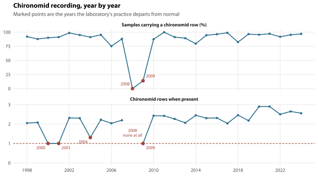
Chironomids — non-biting midges — are the largest single group in these samples and the one whose identification has moved about most. Averaged over the 1,290 edge stream samples taken in the years when recording was normal, they are 14% of the individuals in a sample — the annual mean runs from 8% to 21% — and one to three rows of the family count. Three things happened to them, and all three are visible in Table 3.8.

• 2000 and 2001: family only. Every sample carrying a chironomid carries exactly one chironomid row, where a normal year carries about two — the flat stretch on the dashed line in the lower panel of Figure 3.4. The laboratory was identifying to family and not splitting the sub-families. 2004 is a partial version of the same thing.
• 2008: none at all. Not one of that year’s 43 samples records a chironomid. In 36 samples the following year, 5 do. A group that is a seventh of the animals in a normal sample does not vanish from a whole year’s sampling and come back, so this is either a lost data-entry batch or a change in what the laboratory was asked to identify — and nothing in the archive distinguishes the two (dq:chironomid-absence-2008).
• From about 2010: sub-families, relabelled. Chironominae, Orthocladiinae and Tanypodinae are recorded as separate rows and then relabelled to family level, so Council’s published family count counts one family up to three times. Chapter 1 sets out the mechanism; the effect on the trend is the 0.52 families per decade isolated in Section 3.4 above.

Two consequences travel with these years, and they are easy to miss because they both look like good news.

The family count and %EPT are distorted across 2000–01 and 2008–09. Removing chironomids removes rows from the denominator of %EPT as well as from the family count, so both metrics move, and in the years chironomids are absent they move up. Any n_families or %EPT series crossing those years needs a chironomid-free sensitivity check; n_families_strict and signal2 are unaffected, and are the cross-checks to use.

The four years SIGNAL-SF appears to see the sample best are these years. Chironomidae is the largest single group carrying no SIGNAL-SF grade, so when it is recorded coarsely or not at all, the share of the sample invisible to the index drops for a reason that has nothing to do with grade coverage (chapter 1 plots the series). A model using that column as a covariate is, in those years, partly controlling for identification practice. signal2 has complete coverage and does not have the problem.

3.6 The habitat protocol, and what is recorded by eye

3.6.1 Riffle sampling stopped in 2007

Figure 3.5: Edge and riffle sampling by year. Riffle sampling was routine until 2007 and has effectively ceased since — one riffle sample in the 17 years since, in 2016. The AUSRIVAS edge protocol is the current standard.

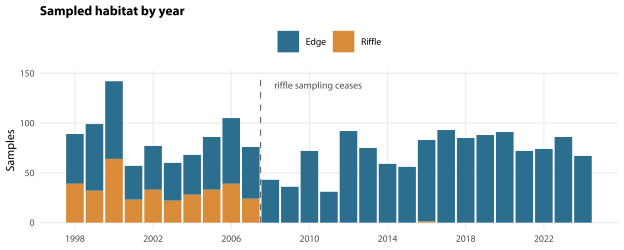
Habitat is coded three different ways in the source data: numeric codes (1 = Riffle, 2 = Edge) before 2006, the strings Edge/Riffle from 2006, and a mixture in 2019–2020 where some rows revert to the numeric code. The water quality database adds a lower-case edge variant. All of these are resolved to a single two-level factor.

Of 2,062 samples, 338 are riffle samples and 1,724 are edge samples. Riffle and edge habitats support different communities, which is why the NSW AUSRIVAS protocol treats them as separate habitats with separate predictive models rather than pooling them (Turak et al. 2004), so mixing them inflates apparent variability. Edge-only is the methodologically consistent series and the default in the shared community_matrix() function; a chapter that includes riffle samples must justify it and show a sensitivity check.

This is the change with the largest single number attached to it, and it is the one most easily missed, because it is not a change in the measurement at all — it is a change in which habitat was measured.

The published rating bands were derived from 2012–2015 percentiles, by which time sampling had been edge-only for five years. So all 338 riffle samples — every one of them from 1998–2007 bar a single sample in 2016 — are scored against a distribution they were not drawn from. Paired within site and year, a riffle sample scores +0.26 factor-score units above the edge sample taken alongside it on the same day (95% CI 0.17 to 0.34, 275 site-years with both habitats sampled, p = \(2.3 \times 10^{-8}\)).

That is a quarter of a factor score of upward bias sitting on the entire first decade of the record and on none of the rest — which is to say it is confounded with the very question of whether waterway health has changed since the 1990s. It pushes the early years up, so it works against the finding of improvement rather than manufacturing it; but a confound that happens to point the helpful way is still a confound, and it has to be handled rather than mentioned.

The handling is one line of code. Filter on health_score$band_applicable, or show the edge-only series as a sensitivity check, and say which you did.

3.6.2 How trustworthy are the habitat records?

Physical habitat is the one block in this report recorded by eye, by different people, over 19 years, against no written protocol — and chapter 9 ranks it first among the things that explain why creeks differ. So it gets the same scrutiny the water quality block gets. Two checks are run on it, and both come back with something.

The habitat records drift within a fixed site. Fitting each variable against the year of description with a site random effect, 10 of the 13 move significantly at a site that did not move; allow each field round its own level as well — which is the right model, because everything described in one round shares whatever that round did — and 7 still do. The estimates barely move either way on 11 of the 13 variables; the exceptions are named in Table 3.9’s caption. Riparian shading, the variable carrying this report’s headline management suggestion, rises by 11.7 percentage points per decade at an unchanged reach, which over the 17 years the shading field has been on the datasheet is a rise of about 20 points. Over the whole description record detritus cover falls by 9.6 points per decade, moss cover by 8.3 and trailing vegetation by 7.6. The four moving together has the shape of a change in the form or the training, not of four independent ecological trends. Because a site mean is an unweighted average over whatever descriptions a site happens to have, sites described mostly early and sites described mostly late are not being compared like with like.

And the form was in fact revised — the database dates the revisions itself. A column empty for every early description and populated afterwards is a field that was added to the sheet; the reverse is a field that was dropped. On that reading tblSiteDescription records three revisions. Six fields appear at once in 2008 — riparian shading, algal cover, flow level and the three channel depths — so the shading series begins with a form change, and there is no pre-2008 shading to compare it with. Three riparian vegetation fields — the percentages under trees below 10 m, shrubs and vines, and grasses and ferns — are recorded until 2018 and never again. In 2024 the single algal cover percentage is replaced by separate filamentous algae and periphyton fields, and the column the old measure was kept in is still called Algae% OLD measure in the database. So the sheet demonstrably changed three times, and you should be able to date the revisions from your own records.

None of the three explains the drift, though. The drift in all four variables is gradual rather than stepped — a changepoint fitted at every candidate year does not beat a straight line for riparian shading — and 2018 and 2024 are too late to account for a rise that is already most of the way there by then. A revision that changed how a retained field was explained, or a change in who was trained and by whom, would leave no trace of this kind in the schema. That is what the drift looks like, and the schema cannot confirm it.

Observer identity is recorded, and it matters. It is easy to assume nobody wrote down who made these visual estimates, because the site description sheet does not ask. But wq$field_officer does record it, and site_description joins to wq on the water quality sample code. The field is populated for 227 of the 1,006 stream descriptions, all between 2018 and 2024, naming 5 officers.

Table 3.9: How much each habitat variable moves within a fixed site over the 2006-2025 description record: a mixed model with a site random effect, so this is drift at a place rather than a difference between places. Not every row spans it — riparian shading and algal cover were added in the 2008 form revision and begin there, which is part of why the Descriptions counts differ. The last two columns add a random effect for the year of description. |t| above 2 is the usual significance mark, and on 11 of the 13 variables it is the t statistics rather than the estimates that move: a field round is one occasion, not thirty independent ones, so the site-only model is too confident about how well the drift is measured. The exceptions are on the page: macrophyte cover and fine sediment — macrophyte cover changes sign on an estimate near zero in both models, and fine sediment’s drift more than triples. Neither carries anything this section concludes.

Variable	Descriptions	Drift per decade	t	Drift, year in model	t
Riparian shading (%)	894	+11.7	9.0	+11.5	5.4
Trailing vegetation (%)	967	-7.6	-5.9	-7.4	-2.7
Bank overhang (%)	969	+4.9	3.7	+6.0	1.5
Riffle (%)	910	+3.7	2.7	+3.1	0.9
Moss cover (%)	958	-8.3	-6.5	-8.1	-2.2
Macrophyte cover (%)	909	-0.3	-0.3	+0.6	0.3
Sedimentation (%)	886	-4.5	-3.2	-4.9	-2.4
Detritus cover (%)	961	-9.6	-8.6	-10.3	-3.3
Algal cover (%)	908	+2.3	1.0	+1.9	0.2
Channel width (m)	853	+0.3	2.7	+0.2	0.7
Substrate coarseness	933	+0.2	3.8	+0.2	2.8
Fine sediment (% silt and clay)	933	-3.1	-4.2	-10.5	-2.1
Bedrock (% of substrate)	933	0.0	0.0	+0.2	0.1

The second question — who wrote the number down — has its own table, Table 3.10, and it is published whole rather than summarised.

Table 3.10: Variance shares from a model with a site and a field-officer random effect, fitted on the 227 stream descriptions that name an officer (2018-2024, 5 officers). The n column is smaller than that on every row: it is the descriptions on which that particular variable is populated. Brackets are 95% parametric bootstrap intervals on the share. The last three columns come from the same model with a year random effect added, which is the only handle these data give on the confounding: each officer works a block of months, so the plain officer column cannot tell a person apart from a season.

Variable	n	Officer	Site	Officer, year in model	Site, year in model	Year
Algal cover (%)	216	24% (1-49)	0% (0-10)	7%	0%	39%
Macrophyte cover (%)	180	22% (0-47)	11% (0-27)	0%	12%	20%
Riffle (%)	205	18% (1-40)	36% (21-51)	4%	39%	16%
Detritus cover (%)	216	15% (0-37)	10% (0-23)	11%	11%	4%
Trailing vegetation (%)	212	13% (0-33)	19% (5-34)	16%	18%	4%
Bank overhang (%)	212	11% (0-28)	20% (6-34)	11%	20%	6%
Channel width (m)	211	8% (0-21)	61% (46-73)	0%	62%	6%
Moss cover (%)	215	5% (0-15)	39% (24-54)	3%	39%	6%
Riparian shading (%)	205	4% (0-14)	48% (32-61)	4%	48%	0%
Sedimentation (%)	171	4% (0-14)	48% (32-63)	4%	48%	0%
Substrate coarseness	206	2% (0-9)	52% (37-65)	2%	49%	10%
Fine sediment (% silt and clay)	206	0% (0-5)	6% (0-21)	0%	7%	32%
Bedrock (% of substrate)	206	0% (0-2)	63% (49-73)	0%	63%	0%

Reading Table 3.10 rather than a count of it: the officer’s share is above the creek’s for 3 of the 13 variables — algal cover, macrophyte cover and detritus cover — and that is the rule “officer share at or above site share”, stated because the answer depends entirely on which rule you use. Loosen it to “officer above 10%” and the answer is 6; ask instead for the variables whose bootstrap lower bound clears half a percentage point and it is 2, algal cover and riffle percentage. That is a cut rather than the more natural “the interval excludes zero”, and deliberately so: a variance share cannot be negative, so the bootstrap piles up against the bound. 7 of the 13 lower bounds are exactly zero and 3 more are positive only in the last decimal the resampling carries — read literally, “excludes zero” would return 6 variables, of which 3 would be arithmetic rather than evidence. With five officers a variance share is not estimated at all precisely, which is what the intervals are there to show.

Two things Table 3.10 says that no single count does. The first is that the intervals are enormous — algal cover’s officer share is 24% with an interval of 1-49% — because five officers is five observations of an officer effect however many descriptions they wrote between them. The second is that most of the officer signal will not stand up to the calendar. Give the year its own term and the officer’s share of algal cover falls to 7% while the year takes 39%, and the number of variables on which the officer beats the creek falls from 3 to 1. Officer and year cannot be separated on this record and Table 3.10 does not pretend otherwise.

What survives all of that is the qualitative point, and it is enough: on 8 of the 13 variables an officer term earns its place in a model that already knows which creek it is (likelihood-ratio p < 0.05), and for riparian shading it earns its place even against site and year together (chi-squared 6.2 on 1 df, p = 0.013; officer SD 4.9 percentage points against a site SD of 16.2). Who holds the clipboard is part of what a visual percentage measures.

One thing this is not. A variance share is not a bias. That algal cover has 24% of its variance sitting with the officer does not make algal cover 24% wrong, and it is not a reason to throw the column away — there is no more accurate version of it to throw it away in favour of. It says that two people looking at the same reach would write down different numbers, which is a statement about how tightly the variable is defined, not about whether it is measuring anything. The fix that follows is a page of worked examples and a half-day together in a creek before each season, not a smaller dataset. Algal cover, macrophyte cover and detritus cover are the ones to start with, and riffle percentage is worth adding for a different reason: the officer’s share of it is large in absolute terms even though the creek’s is larger still.

3.6.3 Testing the shading trend from the air

Officer and period cannot be separated on this record, and no model on these data will separate them. Aerial photography can, because it is independent of every field officer. Your Nearmap subscription carries a historical archive over this LGA, and canopy has been classified in a 30 m buffer around each of 123 located sites from it. The LGA is long enough that a single flight rarely covers all of it, so the series is 17 separate surveys giving one capture per site per year from 2014 to 2021 — 900 site-captures in all — every one of them flown between July and October, so the series is one season and sun angle and phenology are as close to constant as the archive allows. A tight buffer on a mislocated point is noise, so only sites with a position good enough to buffer are used. That turns out not to be the binding constraint: the 44 sites whose positions chapter 4 recovered from stored eastings and northings contribute almost nothing here, because a site that needed its position recovered is generally a site that stopped being described years ago, and the test needs descriptions and imagery from the same year.

What this tests is the trend, not the level. Canopy seen from above is not the same quantity as shade over the water estimated from inside the channel looking up, and on a narrow closed-canopy reach the channel may not be visible from above at all — so the aerial measure is blind exactly where in-channel shading is highest. The two are not expected to agree in absolute terms and they are not asked to.

The aerial measure works, and the first thing it says is that the officers are right about which reaches are shaded. Within a single capture, where the imagery’s radiometry is a constant, a reach the officers called more shaded is measurably greener from above: +0.0129 standard deviations of canopy per percentage point of recorded shading (95% CI 0.0086 to 0.0172, 325 site-captures). The cross-sectional correlation is positive in 11 of the 12 captures large enough to compute one. The visual shading estimate is measuring something real about a reach.

It does not corroborate the trend. Within a site, a year in which an officer recorded more shading than that site’s own average is not a year in which its canopy was above its own average: +0.0006 standard deviations per point (95% CI -0.0036 to 0.0048, 318 site-captures at 55 sites). Measured against the between-site calibration above, that is a ratio of -27.8% to 37.4% — the year-to-year movements in the field record carry at most about a third of the canopy signal that a between-site difference of the same size carries, and are consistent with carrying none of it. Asked the other way, correlating each site’s field shading slope with its aerial slope over 2014–2021: if the field slopes were real vegetation change that correlation would be 39.6%, and it is -11.3% (95% CI -37.7% to 16.8%, 51 sites). Both results hold across 15, 30, 50 m buffers. Over the same window and the same 55 sites the officers recorded shading rising 18.7 points per decade (95% CI 8.1 to 29.3, n = 377), which is steeper than the 11.7 over the whole record.

The same test on all four drifting variables gives the same answer four times. Moss and detritus are in-channel quantities no overhead camera sees directly, but all four are strongly associated with canopy between reaches, and that association is what the test uses. The directions are a check in themselves: trailing vegetation grows where light reaches the bank, so it should run the opposite way from the other three, and it does.

Table 3.11: The four habitat variables that drift, each tested against aerial canopy in the same 30 m buffers. Units are standard deviations of the capture-standardised aerial measure per percentage point of the field variable, with 95% Wald intervals. The between-reach column compares different sites within one capture, where the imagery’s radiometry is constant; the within-reach column compares a site with itself across years, on the 55 sites described in at least three of the aerial years. Every variable is measured well between reaches and none of them moves with the canopy at a fixed reach.

Variable	n (between)	Between reaches	t	Within a reach	t
Riparian shading (%)	325	+0.0129 (0.0086 to 0.0172)	5.9	+0.0006 (-0.0036 to 0.0048)	0.3
Trailing vegetation (%)	332	-0.0116 (-0.0162 to -0.0070)	-5.0	+0.0009 (-0.0029 to 0.0046)	0.5
Moss cover (%)	332	+0.0157 (0.0117 to 0.0197)	7.7	+0.0006 (-0.0035 to 0.0046)	0.3
Detritus cover (%)	326	+0.0076 (0.0016 to 0.0137)	2.5	+0.0037 (-0.0007 to 0.0081)	1.6

One thing the imagery cannot do. There is at most one capture per site per year, so a capture’s radiometry and the calendar year are perfectly confounded — structurally the same trap as officer and period in the field data. The archive is not calibrated between captures, and the capture-to-capture component of the aerial measure (SD 0.0338) is larger than the difference between sites (SD 0.0236). So the question “did canopy rise across the network” cannot be answered from this archive at all. Fitting that model anyway returns a steep fall, -0.068 units per decade at t = -14.2, and that number is the archive getting sharper and bluer over the seven years from 2014 to 2021, not the Blue Mountains losing its trees. It is quoted here only so that nobody fits it later and believes it.

What the test settles is the part that was in dispute: the officers’ year-to-year shading estimates move without the canopy moving with them. The 11.7 points per decade is a change in recording, not a change in the creeks, and nothing in this report should be built on riparian shading having risen.

That is not the same as saying the habitat block is unusable, and chapter 9 shows it is not: rebuilding every habitat site mean from year-detrended values and refitting the variance partition leaves the block’s ranking where it was (Section 9.4). What it does mean is that a block ranked first on visually estimated percentages is not measured as cleanly as one ranked below it on instrument readings, and the worst-affected variables should be read as indicative. Which is exactly what Table 3.11 shows, one row at a time, for all four of the drifting variables, and why chapter 15 declines to put riparian shading into a revised rating.

3.7 What changed in the water quality method

Four things: when in the year the round went out, which probe it carried, what the laboratory could see, and something at the bench in the 6 May 2004–1 February 2005 sampling gap. The first of those is fully correctable and the other three are not, so it goes first and gets the shortest section.

3.7.1 The sampling calendar moved by about 3 months

The median sampling date has moved from 2 March over 1998–2005 to 26 May over 2020–2025 — a drift of 85 days, or about 3 months, out of late summer and into late autumn. It is not monotonic — 1998, whose 25 samples fall in October, November, and December; 2008, whose 27 samples fall in March, April, September, November, and December, so both sit far above the trend — but the direction over the record is unambiguous. This one was not on anybody’s list of things to watch, and it is the largest single confound in the water quality record.

Figure 3.6: The sampling calendar has drifted by about 3 months. Each point is one water quality sample, placed at its day of year; the line joins the annual means and is not a fitted trend. Sampling that used to be done in late summer is now done in late autumn, so a naive comparison of 2024 with 2001 compares autumn water with summer water. Two years sit far above the rest. 1998, whose 25 samples fall in October, November, and December; 2008, whose 27 samples fall in March, April, September, November, and December. Neither was a single late round — both spread across months either side of the mean the line plots, and the higher of the two is the first year of the record, so the line starts at its maximum rather than rising to it.

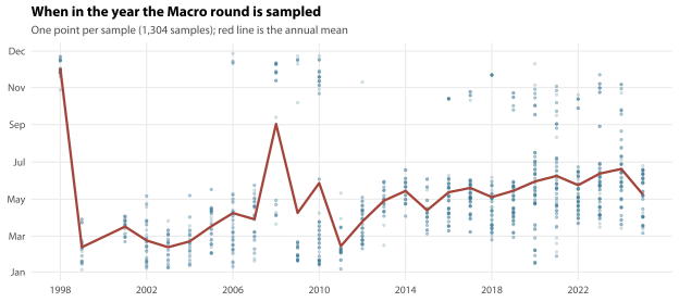
The consequence is direct, and water temperature shows it most cleanly. Fitted with site and year random effects but no seasonal term, water temperature appears to be falling by 1.83 °C per decade. Add the two day-of-year harmonics and the same data say it is rising by 0.58 °C per decade (95% CI 0.31 to 0.85, 1,290 samples). Not a smaller trend, or a less certain one: the opposite sign. This is the clearest demonstration in the book of what the calendar drift does to a naive fit, and it belongs here, in the chapter that dates the drift and sizes it. Chapter 6 reports the temperature trend itself, and reports it from this same fit (Section 6.4.1).

Figure 3.7: Naive against seasonally adjusted temperature trend. Orange points are the raw annual mean water temperature with standard errors; the blue line and ribbon are the fitted trend from a model with two day-of-year harmonics and site and year random effects, evaluated at the mid-record sampling date. The raw series falls because sampling moved from summer to winter; the adjusted series rises.

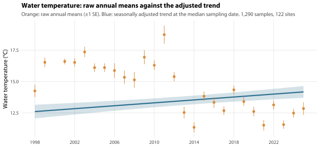
Every water quality model in this report therefore carries two day-of-year harmonics. Where a naive and an adjusted estimate differ materially, both are reported. This one is fully correctable, and it costs nothing.

3.7.2 Two instrument changes, and a laboratory discontinuity

Figure 3.8: Water quality measurements by year, shaded by the multiprobe in use. Any trend crossing 2017 or 2020 may contain a step change caused by the instrument rather than by the environment.

Table 3.12: Water quality samples by instrument era, over all 1,970 samples in the database that carry any measurement. That is the book-wide population and not this chapter’s primary stream set, which is the smaller 1,304 and is broken out by era in the paragraph below. The Device field is populated only from 2020, so the era is derived from the sampling date and cross-checked against Device where present.

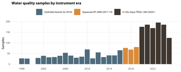
Instrument	Period	Samples
Hydrolab Quanta multiprobe	1998–2016	714
Aquaread AquaProbe AP-2000	2017–2019	224
In-Situ Aqua TROLL 500	2020–present	1,032

The Device column is populated only for the Aqua TROLL era, so the eras are derived from the sampling date and cross-checked against Device where it exists. Every water quality trend crossing 2017 or 2020 has to consider a level shift from the instrument, and every chapter that fits one tests for a step at those dates and reports the result whether or not it finds one.

The probe has been replaced twice (Table 3.12): a Hydrolab Quanta multiprobe until 2016, an Aquaread AquaProbe AP-2000 over 2017–2019, and an In-Situ Aqua TROLL 500 from 2020. In the primary set that is 665, 196 and 443 samples respectively. Within the Aqua TROLL era two serial numbers appear, recorded under 4 different device labels, and they do not agree with each other: on turbidity, unit 743439 returns a reading at or below 0.1 NTU on 28% of visits and unit 855179 on 68%. A further 135 turbidity readings in the primary set carry no device identifier at all.

Every probe-measured parameter is therefore tested for a level shift at 2017 and at 2020, in two independent ways.

• An era term added to the trend model. If the trend estimate collapses when era is included, the trend and the instrument change are not separable.
• A windowed step test: for the three years either side of a boundary, restricted to sites sampled on both sides, a level shift is estimated alongside a linear trend, a seasonal term and antecedent rainfall. This is a within-site before-and-after comparison and is much less vulnerable to the site network changing shape.

The step test is calibrated by running it at 2011 and 2014 as placebo cut points, where no instrument change occurred. A parameter that shows steps at the placebo cuts as well as the real ones is simply unstable on multi-year timescales, and neither its trend nor its steps should be read as environmental.

The laboratory parameters — alkalinity, phosphate, nitrate-N and faecal coliforms — come from test kits and incubation, not the probe, and are not subject to the probe changes. They are still run through the same tests, where the era term is a pure period effect. Any step they show at 2017 or 2020 is evidence that something other than the probe changed at those dates, and is used below as a negative control.

Separately, the faecal coliform record breaks across the 2004–05 summer, by far more than any instrument effect could account for; Section 3.7.6 works out when, how big, and what it was not.

⚠ One of those four laboratory parameters carries an unknown that no instrument history can settle: phosphate’s species is unconfirmed. Nothing in either database or the methods document says whether these readings are phosphate as PO₄ or as P, and the two differ by a factor of three (Section 7.5, dq:phosphate-units). It cancels out of a step, a percentage change or a censored share, which is what this chapter reports phosphate as; where it bites is a phosphate concentration in ppm, such as the detection floors below. Nitrate-N declares its species in its name and phosphate does not.

3.7.3 Level shifts at the instrument boundaries

Figure 3.9: Estimated level shift at four cut points, from a within-site before-and-after comparison over three years either side, controlling for a linear trend, season and antecedent rainfall. 2011 and 2014 are placebo cut points where no instrument change occurred; 2017 and 2020 are the two probe replacements. Bars are 95% confidence intervals from the site random effect model, which treats the samples in a field round as independent and is therefore optimistic; Table 3.13 gives the interval that survives a year random effect as well. Effects are in the parameter’s modelling units, so log-scale parameters are on a proportional scale. Dissolved oxygen (mg/L) and Conductivity (µS/cm) carry the instrument signature — an interval excluding zero at both probe replacements and at neither placebo. Phosphate (ppm, as PO4 or as P) and Nitrate-N (ppm) show the same pattern but are laboratory parameters, measured by test kit and incubation rather than by the probe, so no probe replacement can have produced it — for them the pattern is the negative control firing, and it is evidence that something other than the probe changed at those dates. But 6 of the 22 placebo intervals exclude zero too, in pH, Dissolved oxygen (% sat.), Salinity (PSU), Turbidity (NTU), and Alkalinity (ppm CaCO3), so a step at a real boundary is not on its own evidence of an instrument change; pH excludes zero at all four cut points and is unstable rather than instrument-affected.

Table 3.13: Estimated level shift at each cut point, in modelling units (natural units for temperature, pH and DO; log units for the rest, where 0.69 is a doubling). An asterisk marks an interval excluding zero with a site random effect; a ‘y’ marks one that still excludes zero once a year random effect is added. The bracketed figure is AIC(trend only) minus AIC(step only): positive means the data prefer a step to a gradual change over the window, negative means they prefer a trend.

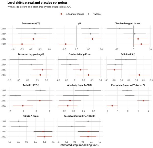
Parameter	Type	2011 (placebo)	2014 (placebo)	2017 (probe)	2020 (probe)
Temperature (°C)	Probe	+0.18 [-1]	+0.23 [0]	+0.13 [0]	-0.49 [0]
pH	Probe	+0.33*y [+8]	+0.34*y [-28]	+0.39*y [-31]	-0.26* [+7]
Dissolved oxygen (% sat.)	Probe	-8.27* [-7]	+0.75 [-2]	+2.68 [+1]	+4.57 [+1]
Dissolved oxygen (mg/L)	Probe	-0.28 [-1]	+0.18 [0]	+0.79* [+8]	+0.66* [+7]
Conductivity (µS/cm)	Probe	+0.01 [0]	+0.04 [-3]	+0.16* [+7]	+0.26* [-1]
Salinity (PSU)	Probe	+0.16* [+3]	+0.02 [-2]	0.00 [-4]	+0.34*y [-5]
Turbidity (NTU)	Probe	+0.33 [-3]	-1.58*y [+27]	+0.28 [-8]	-1.01* [+5]
Alkalinity (ppm CaCO3)	Lab	+0.29* [+2]	+0.04 [-10]	-0.08 [0]	-0.12 [-7]
Phosphate (ppm, as PO4 or as P)	Lab	-0.07 [0]	+0.19 [-6]	+1.49*y [+23]	-1.51*y [+24]
Nitrate-N (ppm)	Lab	-0.47 [+3]	-0.40 [+2]	+0.92* [0]	+1.01* [+1]
Faecal coliforms (CFU/100mL)	Lab	+0.31 [0]	-0.66 [-5]	+0.33 [-4]	+0.31 [-1]

Three cautions belong with Table 3.13 before it is read.

1. A step and a trend are nearly the same regressor over a six-year window. The post indicator and the linear time term correlate at -0.92 to -0.74 in every one of the 44 fits. With no overlap period between instruments these estimates identify that something changed at the boundary far better than they identify its size, which is why the AIC comparison is reported: where a step-only model does not beat a trend-only model, neither reading can be preferred.
2. A single cut cannot be established against year-to-year variation. Three years either side is three annual means either side. Once each year is allowed its own level, only 7 of the 44 shifts survive (the ‘y’ marks): Phosphate (ppm, as PO4 or as P) at 2017, Phosphate (ppm, as PO4 or as P) at 2020, pH at 2011, pH at 2014, pH at 2017, Salinity (PSU) at 2020, and Turbidity (NTU) at 2014. Neither dissolved oxygen step and neither conductivity step is among them — while three of pH’s four, including both placebo cuts, and turbidity’s 2014 placebo step are. A three-versus-three-year difference is not on its own evidence of an instrument change, which is exactly what the placebo cuts were built to show. The argument in this section therefore rests on the placebo comparison — how big a three-versus-three-year difference looks when nothing changed — and on the era terms in the full-record models of Section 6.4.3, rather than on any individual interval here.
3. These are the strongest claims the design can make, and they are weak. Two days of side-by-side operation of the old and new probes would replace every one of them with a measured correction factor.
4. Nothing in this chapter is corrected for multiplicity, and the placebo cuts are the reason. This section alone reports 44 shift estimates — 11 parameters at 4 cut points — each in three forms, and the chapter reports many more verdicts elsewhere in several different currencies. None of them is Benjamini–Hochberg corrected. Other chapters do control the false discovery rate, wherever the family is a scan — a set of tests run in order to find which of its members are significant, of which the water quality chapter’s site-by-parameter trends
   1. are the largest in the report. There is no such family here — the cut points and the parameters were both fixed before any of it was fitted, and every one of them is reported. What is used instead is a measured null. 2 of the 4 cut points are places where nothing happened, so how often this test fires with nothing to find is observed rather than assumed — which is what a correction is trying to approximate, and it is why point 2 above reads the way it does. It is a control on the section, not on any single row of it. A lone parameter read off Table 3.13 on its own carries no protection at all, and none of the verdicts here is intended to be read that way.

Read down Table 3.13, three patterns emerge.

Clean instrument signature — dissolved oxygen and conductivity. Dissolved oxygen steps up at 2017 and again at 2020, steps at neither placebo cut, and prefers a step to a trend at both real cuts (ΔAIC +8 and +7). Conductivity steps at 2017 and prefers a step there (ΔAIC +7), but at 2020 a trend fits it as well as a step (ΔAIC -1), so only the 2017 conductivity step is supported. Dissolved oxygen gains 0.79 mg/L at the Aquaread changeover and a further 0.66 mg/L at the Aqua TROLL changeover — together about 1.45 mg/L. The whole apparent change in dissolved oxygen over the 27.0 years of record is about 0.64 mg/L, so the two instrument steps together are larger than the entire apparent improvement. The published sensor comparisons do not support the simplest explanation for that, and it is worth saying so. Optical and Clark-cell membrane sensors read the same water to similar accuracy when both are freshly calibrated: in a side-by-side field deployment Johnston and Williams (2006) found no systematic offset between the two types against Winkler titrations. What they did find is a large difference in drift — the membrane sensors accumulated fouling drift of 0.17 to 0.37 mg/L between servicings while the optical sensors drifted by 0.02 mg/L or less. A membrane probe read in the field days or weeks after its last calibration therefore tends to read low, and replacing it with an optical probe removes that downward bias. The size of the steps here, about 1.45 mg/L in total, is of the order that servicing interval alone could produce. That is a mechanism you can check against your own calibration records, and it is a different remedy from a fixed correction factor.

There is a second candidate explanation, and it has been tested rather than argued about. The Aqua TROLL era begins in 2020, which is also when the weather turned: flow state at the time of sampling — recovered from the field sheet in Section 6.7 — is markedly higher from 2020 on, and flowing water is better-oxygenated water. Refitting these step models with flow state controlled removes only a small part of each dissolved oxygen step (Section 3.7.4), so the instrument reading survives the test, and it was a test the record could have failed.

Unstable rather than instrument-affected — pH. pH steps at all four cut points, including both placebos, and the steps change sign. It is also the one parameter that clearly prefers a trend to a step at both 2014 and 2017 (ΔAIC -28 and -31), which is a stronger statement of the same reading: pH is not stepping at boundaries, it is wandering continuously. Nothing about pH in this record is stable on a five-year timescale, so neither its trend nor its steps carry information about the creeks.

A laboratory excursion, not a probe effect — phosphate and nitrate. Phosphate jumps +345% at 2017 and falls -78% at 2020, returning almost exactly to where it started, and nitrate rises at both. Phosphate is a test-kit measurement and cannot be affected by a probe replacement. The censoring rate tells the same story: the share of phosphate results below the detection limit was 75%-89% in 2013–2016, fell to 17%-34% over 2017–2019, and returned to 61%-90% from 2020. The 2017–2019 nutrient results are not comparable with the rest of the series, and the most likely explanation is a change of test kit or reagent batch over those three years. This is a finding about the laboratory, and you can check it against your own purchasing records.

3.7.4 Does it change the dissolved oxygen instrument reading?

Section 3.7.2 reads the dissolved oxygen record as carrying two instrument steps, at 2017 and 2020, whose combined size exceeds the entire apparent improvement over the whole water quality record. If the Aqua TROLL era is also the wet era, part of that step could be water rather than probe. Refitting the windowed step test on the samples that carry a flow state, with and without a flow term, answers it directly.

Table 3.14: The windowed step test of Section 3.7.2, refitted on the subset of samples carrying a flow state so that the two columns are the same samples. Both fits carry site random effects, a linear trend, two seasonal harmonics and 90-day antecedent rainfall. Controlling for flow state removes only a small fraction of each step.

Parameter	Cut point	n	Step, no flow term	Step, flow controlled (95% CI)	Share of step attributable to flow
Dissolved oxygen (mg/L)	2017	268	+0.799	+0.684 (0.125 to 1.242)	14%
Dissolved oxygen (mg/L)	2020	355	+0.678	+0.646 (0.120 to 1.173)	5%
Dissolved oxygen (% sat.)	2017	269	+2.864	+2.512 (-3.610 to 8.634)	12%
Dissolved oxygen (% sat.)	2020	355	+5.299	+5.190 (-0.099 to 10.478)	2%

The instrument reading survives. Controlling for flow state (Table 3.14) reduces the 2017 dissolved oxygen step from 0.799 to 0.684 mg/L and the 2020 step from 0.678 to 0.646 mg/L. Flow state accounts for 14% of the first and 5% of the second. The steps are not the weather, and Section 3.7.2’s conclusion — that the two probe replacements, not the creeks, produce most of the apparent dissolved oxygen improvement — stands unchanged.

Two things follow. First, flow state is a partial answer to the visit-level variation the water quality chapters cannot otherwise explain — but a partial one, because it predicts dissolved oxygen strongly and almost nothing else. Second, the field is now good enough to be worth improving: a dropdown rather than a text box, and the numeric velocity on every visit rather than one in five. Going from an ordinal six-point scale to a measured velocity is what would let this analysis be done properly rather than recovered.

3.7.5 How much of this is the substituted detection floor?

Non-detects are substituted at a floor rather than dropped in seven of this chapter’s eleven water quality parameters, all seven of them modelled on the log scale. Table 3.15 gives each floor and where it comes from. Only one of those seven floors is a confirmed measurement limit — faecal coliforms, at the 10 CFU/100 mL the field notes record (Section 3.7.6). Of the rest, two are laboratory detection limits the data layer inferred and does not confirm, and four are not detection limits at all but substitution points chosen by this analyst. Because the response is logged, the floor sets the value of every censored point and therefore the slope. That substitution is done here only so that the sensitivity below can be shown; it is not defensible as an analysis in its own right. Helsel (2006) demonstrates that substituting a fraction of the detection limit invents structure that is not in the data and distorts means, variances and regression slopes by amounts that depend on the substitution chosen — which is exactly what Table 3.16 measures on your own record.

Table 3.15: All seven substituted floors, where each comes from, and the share of that parameter’s readings it touches. Of these, three are laboratory detection limits carried by the data layer and four are substitution points chosen here rather than limits at all; exactly one is confirmed. Substitution is at the limit rather than at half of it, which is the conventional default; Table 3.16 shows what that choice is worth.

Parameter	Floor	Binds on	Provenance
Faecal coliforms	10 CFU/100 mL	43%	Data layer wq_detection_limits, documented, confirmed = TRUE. The field notes record the laboratory arithmetic — a 1 mL and a 10 mL aliquot plated and multiplied by 100 and by 10 — so 10 is the smallest number the method can produce (Section 3.7.6). This is the only floor in the chapter, or in the book, with a documentary basis.
Phosphate	0.01 ppm	54%	Data layer wq_detection_limits, inferred from the reporting grid, confirmed = FALSE. No phosphate or nitrate-N value below 0.01 ppm exists in the raw table in any year; where a sample carries one reading the smallest positive value of either parameter is 0.01 ppm, and the grid steps in 0.01 throughout, so the floor never moved. The ten values in wq that sit under the grid (2012 only) are laboratory duplicates averaged rather than readings, and count as censored. What the grid fixes is the resolution the results were recorded at, not the floor of the kit that produced them — see dq:lab-detection-limits.
Nitrate-N	0.01 ppm	4.7%	As above, inferred from the same grid and unconfirmed; its three sub-grid values are the same kind of replicate average.
Turbidity	0.1 NTU	23%	No documentary basis. Turbidity is a probe reading with no detection limit in any documentation; 0.1 NTU is this analyst’s choice and is about 1,200 times the smallest positive value recorded. It is also the substituted floor that binds on the most readings.
Alkalinity	1 ppm	0.4%	No documentary basis, and chosen against the data layer’s judgement. Alkalinity is a laboratory parameter, but wq_detection_limits declines to infer a limit for it — “no detection limit inferred; only 4 exact zeros, so the pattern is not diagnostic” — so the 1 ppm floor is this analyst’s, not the layer’s.
Conductivity	1 µS/cm	0.0%	No documentary basis. Effectively uncensored, so the choice does not matter.
Salinity	0.005 PSU	0.1%	No documentary basis. Effectively uncensored, so the choice does not matter.

Table 3.16: Seasonally adjusted trend per decade under four choices of substitution floor, with the floor itself in brackets. An asterisk marks an interval excluding zero. All three parameters are disqualified on other grounds, but the size of the estimate is a property of the substitution as much as of the water.

Parameter	Floor x0.1	Floor x0.5 (DL/2)	Floor as used	Floor x2
Turbidity (NTU)	-82%* (0.01)	-76%* (0.05)	-72%* (0.1)	-67%* (0.2)
Phosphate (ppm, as PO4 or as P)	-59%* (0.001)	-44%* (0.005)	-35%* (0.01)	-27% (0.02)
Faecal coliforms (CFU/100mL)	-9% (1)	-29%* (5)	-28%* (10)	-25%* (20)

The estimated turbidity and phosphate declines move by tens of percentage points across defensible floors, and for phosphate and faecal coliforms alike the choice of floor decides whether the interval covers zero — phosphate’s loses its asterisk at 2x the floor used and the coliform one at 0.1x. Turbidity is the only one of the three whose interval excludes zero at every floor tried. None of these numbers is a measurement of the water in the way a reader will assume. Coliforms are the least bad of the three, because for them we now know which floor is right; but knowing the floor is not the same as knowing the values, and Section 3.7.6 shows that fitting the non-detects as non-detects, rather than substituting anything for them, puts the coliform interval back across zero. All three should be read through the exceedance framing of Section 7.4, not as level trends — which is what this chapter suggests for them anyway. The practical consequence is dq:lab-detection-limits: for phosphate and nitrate, a reported zero and a “below 0.01 ppm” are different data and are still indistinguishable.

3.7.6 The faecal coliform break

Somewhere between the last coliform sample of 2004 and the first of 2005, the numbers fall by about a hundredfold and never come back. Coliform counts from before that point are not the same measurement as coliform counts from after it, and running them together as one series produces an improvement large enough to swamp everything else in the water quality record.

Figure 3.10: Faecal coliform counts by year, on a log scale, as the geometric mean of that year’s Macro stream samples. Counts fall about a hundredfold across the 2004–05 gap in sampling and never return. The fall is the same size at every site, reference creeks included, which is why it is read as something that happened at the bench rather than in the water.

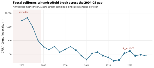
3.7.6.1 When it happened

Fitting the break rather than eyeballing it puts it at 2004.50, with everything from 2004.25 to 2005.00 fitting about as well. That interval is not really a statistical result: it is the hole in the sampling. The last coliform sample before the break is 6 May 2004 and the next one is 1 February 2005, a gap of 9 months, and no test can place a step inside a window with no data in it. The break is somewhere in that gap and cannot be dated more precisely than that.

What can be said is that 2005 is on the far side of it. Of the 13 coliform readings taken in 2005, 11 are already at post-break levels; the exceptions are two readings on one day, 13 April, of 3,900 and 6,300 CFU/100 mL. Those two are what lift 2005’s annual geometric mean to 94 CFU/100 mL, against 985 in 2004 and 34.5 in 2006. So neither “the series breaks in 2005” nor “the series starts in 2006” is a statement about when the measurement changed. It changed somewhere in that 9-month gap, and that is as close as the record allows anyone to put it.

3.7.6.2 How big it is

Across the 33 sites measured on both sides — which is the comparison to make, because which sites were sampled changes from year to year — and with month of year and year-to-year variation both allowed for, the drop is 1.90 on a log₁₀ scale (95% CI 1.69 to 2.11). In plain terms: counts fall about 79-fold, and anywhere from 48-fold to 129-fold is consistent with the data.

That interval sits comfortably around an exact factor of 100 (p = 0.35) and rules out both a factor of 10 and a factor of 1,000 decisively (p < 0.001 for each). A round hundred is the number to carry around, and it is a suggestive one: a hundred is what you multiply a 1 mL plate count by.

3.7.6.3 It is not the creeks

The drop happens at every one of the 33 paired sites, and by much the same amount at each. Site-to-site the estimated steps have a standard deviation of 0.58 on the log₁₀ scale, and the standard deviation you would expect from sampling noise alone, if the true step were identical everywhere, is 0.60. Formally, letting the step vary by site does not improve the model (p = 0.32). Taking each site on its own, the median fall is 118-fold at urban sites and 146-fold at the reference creeks, whose catchments have no sewerage, no stormwater and no houses in them — if anything larger in the bushland. (These raw site medians run above the 79-fold pooled figure because the pre-break samples were all taken in the warmer half of the year, which the pooled model allows for and a raw median does not.)

This is the test that matters, and here is why. Something happening in the catchments — a tranche of sewer reticulation going in, an overflow being fixed — hits particular creeks on particular dates by different amounts. Something happening to the measurement hits every sample at once by the same factor. What we see is the second. A hundredfold improvement in undeveloped bushland, on the same date as everywhere else, is not an environmental result.

3.7.6.4 It is not a units slip either

The obvious suspect, given the data is hand transcribed, is a decimal point: CFU/mL against CFU/100 mL is exactly the factor of 100 we are looking at. The numbers rule it out.

The method plates a 1 mL and a 10 mL aliquot and multiplies the colonies counted by 100 and by 10 — three field notes say so in as many words, including one from July 2024 reading “0 colonies in 10ml but 1 in 1ml sample” against a recorded value of 100. Every number in the series is therefore a colony count times 10 or times 100, and lands on a grid of 10s and 100s. It does, on both sides of the break: 76% of the pre-break values are multiples of 10, against 83% after.

Now suppose the pre-break numbers were post-break-style numbers with two extra zeros on them. Then they would have to be multiples of 1,000. Only 3 of 85 are. Put the other way round: the median pre-break reading is 1,870 CFU/100 mL on a grid of 10, so it is resolved to about 0.5% of its own size, where the median post-break reading of 30 is resolved to about 33%. The early numbers carry two more significant figures than a rescaled late number could. They are counts of a few hundred colonies on a crowded plate, not counts of three with a decimal point in the wrong place.

3.7.6.5 So what was it?

Something changed about what was being counted, or how. Divide the numbers through by the plate volume and the early samples imply a median of about 187 colonies on a 10 mL plate against about 3 afterwards — and a note from March 2005 records plates simply “tntc”, too numerous to count. Plates that crowded, at reference sites in bushland, suggest the early counts were picking up something the later ones were not: a switch from total coliforms to thermotolerant ones, a change of medium or incubation temperature, a change of holding time before plating, or a change of laboratory would each do it. The data cannot tell us which, and we should not pretend otherwise.

What would settle it is a records request, and it is worth making: the laboratory’s method log or standard operating procedure for 2003–2006, the analysis reports or invoices for those years, and the original field sheets for the summer of 2004 and the summer of 2005. Any one of them would probably name the change in a line.

3.7.6.6 And after the break, the floor decides the answer

The break is the big problem, but there is a smaller one underneath it, and it is the reason Section 3.7.5 says coliforms are the least bad of three bad cases rather than a good one. From 2006 onward, 47% of the 941 readings are below the detection limit, so whatever number is substituted for them sets the slope.

Substituting at the documented limit of 10 gives a trend of -28% per decade (-43% to -8%); substituting at 1 gives -9% (-41% to +41%). And fitting the non-detects as non-detects — a left-censored model that never invents a value for them at all — gives -22% (-46% to +13%). That last fit cannot carry a site or year random effect, so it is a check rather than the answer, but the check is the one that matters: the interval covers zero. Knowing which floor is right is not the same as knowing the values, and there is no established post-2006 coliform trend to report.

3.8 The one thing worth doing about all this

Most of what this chapter describes is history and cannot be undone. One thing can be, and it is the cheapest suggestion in the report, so it gets its own section: it is easy to read past.

Whenever an instrument or a method is replaced, run the old one and the new one side by side for one round.

Here is what its absence has cost so far. Chapter 6 analyses eleven water quality parameters over 27 years and can confirm a trend in exactly one of them. That is not because the creeks are static. It is because the probe was replaced twice with no overlap at either changeover, so dissolved oxygen gains 0.79 mg/L at the first change and a further 0.66 mg/L at the second — together more than the whole apparent improvement over the record — and nothing in the data can say how much of that is water. The likeliest mechanism is not that optical sensors read high: the published side-by-side comparison finds no systematic offset between the two types, but does find that membrane electrodes drift low between servicings, by 0.17 to 0.37 mg/L in Johnston and Williams (2006)’s field trial against 0.02 mg/L for optical. Replacing one therefore removes a downward bias of about the size seen here. Either way it is the instrument.

Turbidity is worse, because the Aqua TROLL era is not even one instrument. Two serial numbers appear under 4 different device labels; they disagree with each other so strongly that one reads at or below the working floor on 28% of visits and the other on 68%; and a further 135 readings carry no device at all. The site median falls 4.73 to 0.058 NTU across the two changeovers, at 54 of 55 sites. Turbidity has effectively been abandoned as a series.

Two field rounds with both instruments in the car, at a spread of sites, would have replaced every one of those sentences with a correction factor. The next probe replacement is the opportunity, and it will be missed by default unless the overlap is written into the procurement. The same principle applies at the bench: a reagent or test-kit change wants a run of split samples measured both ways, and the 2017–2019 nutrient excursion is what its absence costs.

There is a second, even cheaper habit that would have prevented half of this chapter, and it is simply writing the change down. A dated line in a register — “pick count raised to 200 from this round”, “new phosphate kit, supplier X, limit 0.01” — would have turned four of the eight rows in Section 3.2 from confounds into covariates.

3.9 What this chapter cannot tell you

1. None of these diagnoses can be confirmed against a document, because no document has been found. Every one is an inference from the pattern in the numbers: a step at every site at once, a count that doubles, a group of taxa that disappears for a year. The inferences are strong — a hundredfold improvement in undeveloped bushland on the same date as everywhere else is not a plausible environmental result — but they are inferences, and any one of them could be settled or overturned by a piece of paper. That is why the data section above leads with the paper.

2. A confound measured once cannot be sized, only detected. With no overlap period, the step tests identify that something changed at a boundary far better than they identify how much. Over a six-year window a step and a trend are nearly the same regressor, and only 7 of the 44 shifts survive giving each year its own level. The argument rests on the placebo comparison and on the era terms, not on any single interval.

3. The habitat officer analysis rests on 5 officers and 227 descriptions, all from 2018–2024, which is why every share in Table 3.10 carries an enormous interval. Before 2018 the officer is not recorded at all, so for most of the record the observer can be ruled out but never modelled.

4. The aerial test covers 2014–2021 only, and it tests the trend, not the level. Canopy seen from above is not shade over the water estimated from inside the channel, and the archive is not calibrated between captures, so it can say the officers’ year-to-year movements do not track the canopy and it cannot say what canopy did across the network.

5. This chapter does not attempt to correct the record. It says which corrections are available and what each costs. Applying them is each chapter’s own job, and the reason is that the right correction depends on the question: rarefaction is right for a richness trend and wrong for a rating, an era term is right for a trend and useless for a single year’s report card.

6. Nothing here says the monitoring was not worth doing. A 27-year record with eight reconstructed method changes is still a 27-year record, and it is more than almost any comparable program in New South Wales has. The point of the chapter is to say which questions it can answer, not to suggest it should not have been collected.

Cao, Yong, Charles P. Hawkins, and Mark R. Vinson. 2003. “Measuring and Controlling Data Quality in Biological Assemblage Surveys with Special Reference to Stream Benthic Macroinvertebrates.” Freshwater Biology 48 (10): 1898–911. https://doi.org/10.1046/j.1365-2427.2003.01123.x.

Doberstein, Craig P., James R. Karr, and Loveday L. Conquest. 2000. “The Effect of Fixed-Count Subsampling on Macroinvertebrate Biomonitoring in Small Streams.” Freshwater Biology 44 (2): 355–71. https://doi.org/10.1046/j.1365-2427.2000.00575.x.

Gotelli, Nicholas J., and Robert K. Colwell. 2001. “Quantifying Biodiversity: Procedures and Pitfalls in the Measurement and Comparison of Species Richness.” Ecology Letters 4 (4): 379–91. https://doi.org/10.1046/j.1461-0248.2001.00230.x.

Growns, Jane E., Bruce C. Chessman, Jean E. Jackson, and David G. Ross. 1997. “Rapid Assessment of Australian Rivers Using Macroinvertebrates: Cost and Efficiency of 6 Methods of Sample Processing.” Journal of the North American Benthological Society 16 (3): 682–93. https://doi.org/10.2307/1468153.

Helsel, Dennis R. 2006. “Fabricating Data: How Substituting Values for Nondetects Can Ruin Results, and What Can Be Done about It.” Chemosphere 65 (11): 2434–39. https://doi.org/10.1016/j.chemosphere.2006.04.051.

Hurlbert, Stuart H. 1971. “The Nonconcept of Species Diversity: A Critique and Alternative Parameters.” Ecology 52 (4): 577–86. https://doi.org/10.2307/1934145.

Johnston, Matthew W., and John S. Williams. 2006. Field Comparison of Optical and Clark Cell Dissolved Oxygen Sensors in the Tualatin River, Oregon, 2005. Open-File Report Nos. 2006-1047. U.S. Geological Survey. https://doi.org/10.3133/ofr20061047.

Ostermiller, Jeffrey D., and Charles P. Hawkins. 2004. “Effects of Sampling Error on Bioassessments of Stream Ecosystems: Application to RIVPACS-Type Models.” Journal of the North American Benthological Society 23 (2): 363–82. https://doi.org/10.1899/0887-3593(2004)023<0363:EOSEOB>2.0.CO;2.

Turak, Eren, Natacha Waddell, and Glenn Johnstone. 2004. New South Wales (NSW) Australian River Assessment System (AUSRIVAS) Sampling and Processing Manual. Department of Environment; Conservation (NSW), for the National River Health Program. https://ausrivas.ewater.org.au/index.php/resources2/category/10-manuals?download=15:nsw-sampling-and-processing-manual-pdf-32mb.

Vinson, Mark R., and Charles P. Hawkins. 1996. “Effects of Sampling Area and Subsampling Procedure on Comparisons of Taxa Richness Among Streams.” Journal of the North American Benthological Society 15 (3): 392–99. https://doi.org/10.2307/1467286.