8 What lives in the creeks, and how that changed
Blue Mountains City Council Healthy Waterways — statistical analysis
8.1 What this chapter answers
You asked whether the animal communities in Blue Mountains creeks have changed, whether particular families are becoming more or less common, and what that change is associated with. This chapter answers all three, on 1,502 edge samples from 125 stream sites between 1998 and 2024 — 26 years of the macroinvertebrate record — covering 117 families.
It also settles a question chapter 5 could not. Chapter 5 found that the raw number of families per sample rises across the record, but that once every sample is standardised to the same number of individuals there is no net trend across the record: the apparent gain in richness is a counting artefact, because the laboratory is processing roughly twice as many animals per sample as it used to (chapter 3, Section 3.4). What chapter 5 could not then say is whether the fall in family counts since about 2010 is good news or bad.
Composition analysis mostly escapes that problem, because it is built from proportions rather than counts. “Mostly” is doing real work in that sentence, and Section 8.3 says exactly how much.
One number in this chapter is worth more than the rest. Tolerant families have given way to sensitive ones. It is the largest and most robust signal anywhere in the monitoring record — and it is the signal your current rating reports worst, for a reason that is structural rather than accidental (Section 8.6).
1. Has community composition changed? Yes, decisively, and in a consistent direction. In the average sample the share of individuals belonging to pollution-tolerant families fell from 42% in 1998–2004 to 17% in 2018–2024, while the share belonging to sensitive families rose from 46% to 64%. (Every sample counts once, so a large sample does not outweigh a small one. Pooling all animals instead gives the same story: 40% to 15%.) These are proportions, so they are very largely unaffected by how many animals were picked from each sample: take a random subsample of a constant 50 individuals from every sample big enough to supply one and the same figures are 40% falling to 16%; at a constant 100 individuals, 40% falling to 14%. Formal testing (Section 8.4.1) confirms a compositional shift over time that is independent of sampling effort, season and site.
2. Is the fall in family counts since 2010 recovery or degradation? Recovery. Chapter 5 asked precisely this. Since 2010 the number of families per sample has fallen in the edge stream samples analysed here (Section 8.5 gives the rate) — and the largest single part of that loss is of tolerant families. (The best estimate is about three fifths of it; a creek-level bootstrap puts that anywhere from two fifths to all of it, so “most” is the likeliest reading rather than an established one, and Section 8.5 gives the interval.) Sensitive families have not declined at all (Section 8.5). The rest is families of intermediate sensitivity, and on a model that allows for year-to-year variation that part of the loss is not established. Creeks are carrying fewer kinds of animal, and the kinds they have demonstrably lost are the ones that indicate poor water.
3. Which families are winners and losers? Of the 75 families common enough to test, 17 show a change in how often they are found that survives control of the false discovery rate, of sample size and of year-to-year variation, and more are spreading than retreating in occupancy — while in relative abundance more are falling than rising. Both measures point the same way about which families: the 6 fastest-spreading families are all mayflies, stoneflies or caddisflies, and 7 of the 12 spreading families are. The ones becoming less widespread are led by mosquitoes and water striders (Section 8.6).
4. What is it associated with? Overwhelmingly, which creek it is. Creek identity accounts for more than forty per cent of what distinguishes one sample from another, dwarfing everything else. Among the things that can actually be measured, catchment imperviousness and geography together explain about twice what the passage of time explains, and climate explains least of all (Section 8.8).
8.2 The data behind this chapter
Each question and request below is set out again in What we need from you, with what it blocks, what an answer is worth and what it would cost you to find, ranked against every other ask in the report.
8.2.1 What this chapter uses, and where it came from
Everything in this chapter runs on one matrix — 1,502 edge samples from 125 stream sites, 1998 to 2024, holding 117 macroinvertebrate families — and every number in it counts individuals or families in that matrix.
Built by community_matrix() on its defaults: edge habitat, family-level identifications only, microfauna dropped. Wetland samples are removed, because a wetland assemblage is a different assemblage rather than a degraded stream one — leaving them in makes the first ordination axis a stream-versus-wetland axis and nothing else. Wetlands are analysed on their own in chapter 11. Relative abundance is the primary form: every individual contributes to a proportion rather than to a total, which is what makes the chapter robust to the pick-count problem.
Blocks: Nothing — this is a statement of what we used. Value: moderate. Costs you: minutes. Refer to it as
dq:composition-analysis-set.
Where this chapter counts families it uses the strict count — chironomids excluded at every label — and not the n_families figure your rating is scored on.
The two differ mainly in how the relabelled chironomid subfamilies are treated: the published count can score one animal group several times. Nothing in this chapter reproduces or reviews the rating, so the strict count is the right one, and it is used consistently. Chapter 3 separates the two and quantifies what the difference costs. The consequence worth knowing is that a richness number here will not equal the same-sounding number in the rating chapters, and neither is wrong.
Blocks: Nothing — this is a statement of what we used. Value: moderate. Costs you: minutes. Refer to it as
dq:strict-family-count-here.
8.2.2 What is wrong with it
Riffle sampling ceased after 2007, and riffle assemblages differ systematically from edge ones, so every composition result here is an edge-habitat result and the 338 riffle samples are excluded outright.
Including them would confound habitat with time, which is the exact confound this chapter exists to avoid: the riffle samples are all early, so a habitat difference would be read as a change over time. The cost is that nothing here describes riffle communities, and riffles are where the most sensitive families live.
Blocks: Any statement about riffle communities, and any comparison of the pre-2008 and post-2008 record that does not hold habitat fixed. Value: moderate. Costs you: minutes. Refer to it as
dq:edge-only-after-2007.
The variance partition in this chapter needs a delineated catchment, a site description and a climate record together, and only 90 of the 125 creeks carry all three, so that section describes the modern monitoring network rather than the whole record.
The variable is total catchment imperviousness, built in chapter 4 from road-corridor polygons and address points rather than measured. It is good enough to rank creeks against one another and not good enough to set a threshold on. The creeks without a catchment are mostly the retired legacy sites, so the partition is also weighted towards the sites you still visit.
Blocks: Reading the driver ranking as a statement about the whole record rather than about the modern network. Value: moderate. Costs you: minutes. Refer to it as
dq:imperviousness-modelled-coverage.
Taxa identified only to order or class — oligochaete worms, mites, microcrustacea, and chironomids at every label — are dropped from this chapter’s matrix in every year, which loses a classic tolerance indicator.
An ordination that mixes family-level and order-level records confounds taxonomic resolution with composition, so the strict matrix is the right choice. It also has one useful side effect. Chapter 3 shows chironomids were recorded to family only in 2000-01 and not at all in 2008; because they are excluded in every year here rather than in the years the practice differed, that gap cannot produce a step in any series in this chapter. The loss is real all the same — oligochaete worms would be informative about the tolerant end of the shift and are simply absent.
Blocks: Reading the tolerant end of the composition shift as if it included worms and midges. It does not. Value: moderate. Costs you: minutes. Refer to it as
dq:order-level-taxa-excluded.
The samples that recorded no animals at all cannot appear in a composition analysis, because a community with no members has no composition, and they are excluded here by min_sample_total.
They are documented in chapter 1. Worth flagging because an empty sample is not the same as a missing one: it may be a genuinely barren reach, a failed sort, or a sheet that was never filled in, and the three would be read very differently.
Blocks: Nothing in this chapter, but it bears on any count of “samples analysed”. Value: low. Costs you: minutes. Refer to it as
dq:empty-samples-cannot-appear.
8.2.3 Questions only you can answer
Was SIGNAL-SF chosen over SIGNAL 2 for a reason we should know about — a comparability requirement, an agency expectation, an agreement with someone — or was it simply the version in use when the rating was built?
It matters because this chapter’s strongest result is that SIGNAL-SF is structurally the less able of the two to see the change that has actually happened in these creeks: it has no grade for the worms, the chironomid subfamilies and the mites that dominate a degraded sample, and it grades mosquitoes and water striders as though they were clean-water animals. Swapping the factor is a real option, and knowing why the original choice was made would tell us what it would cost you elsewhere.
Refer to it as
dq:signal2-as-a-rating-factor.
Two sensitive families run against the general recovery — the stonefly Notonemouridae and the damselfly Synlestidae are both becoming less widespread. Does that match what your field staff see?
Everything else in this chapter says sensitive families are gaining ground, and these two are the exceptions that survive a fully corrected model. They may be a genuine local loss worth acting on, or they may be an identification habit. Field recollection would tell us which is worth chasing before we spend any more analysis on it.
Refer to it as
dq:sensitive-family-decliners.
Were terrestrial and semi-terrestrial animals — Oniscidae and Talitridae, 21 samples each — always recorded when they turned up, or did the instruction change at some point?
Both families appear to decline over the record. Whether that is an animal or a convention we cannot tell from the data, and one long-serving officer’s recollection would settle it in a minute.
Refer to it as
dq:terrestrial-taxa-convention.
8.4 Has composition changed?
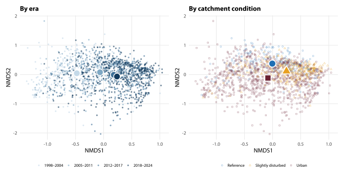
The standard way to look at whole communities at once is an ordination: every sample becomes a point on a map, and points close together are samples with similar animal communities. The map has no units and its axes mean nothing individually; only the distances between points matter. The method here is non-metric multidimensional scaling on Bray–Curtis dissimilarities, the long-established default for assemblage data because it assumes nothing about the community responding linearly to anything (Clarke 1993).
Read that as an impression, not as evidence. Stress — how much a multi-dimensional pattern has to be distorted to fit on a flat page — is 0.164 in three dimensions and 0.237 in two, which is the honest cost of putting 1,502 heterogeneous samples on one map (below about 0.20 is the usual rule of thumb for a usable picture (Clarke 1993)). Neither solution reached a repeated convergent minimum after 30 and 30 random starts, which is normal at this size; the figure is the best of that many starts, not a demonstrated optimum, and a different seed would nudge it. The method note is on this chapter’s data list. Nothing in the rest of the chapter depends on the ordination — every test below works on the full distance matrix with no map involved.
8.4.1 Testing it
An ordination is a picture, not a test. PERMANOVA (Anderson 2001) asks whether samples grouped one way (by era, by catchment condition) really are further apart than samples grouped at random. It works directly on the dissimilarity matrix and gets its p-values by permutation, so it needs no assumption of multivariate normality — which assemblage data never satisfy.
The complication is that these 1,502 samples come from only 125 sites, and repeated visits to the same creek are not independent observations. Treating them as independent would make any test wildly over-confident. Two separate designs are therefore used.
- Within-site design. Every sample is used, site is fitted first so that everything after it is tested on variation within creeks, and permutations are restricted to stay within a creek. This is the correct test for time, season and sampling effort. The site term’s own share of the variance is reported but it cannot be tested under this scheme, because shuffling samples within a creek never changes which creek they came from.
- Between-site design. Each creek is reduced to a single average community — one row per site — and the test is run on those rows — one per creek. This is the honest sample size for anything that does not vary within a creek, such as its catchment condition or its altitude.
| Term | df | Variance explained | Pseudo-F | p |
|---|---|---|---|---|
| Site (creek identity) | 124 | 43% | 8.9 | not testable |
| Individuals processed (log) | 1 | 1.2% | 29.5 | < 0.005 |
| Season | 3 | 1.6% | 13.9 | < 0.005 |
| Time (decades) | 1 | 0.8% | 21.7 | < 0.005 |
| Residual | 1372 | 53% | – | – |
| Term | df | Variance explained | Pseudo-F | p |
|---|---|---|---|---|
| Catchment disturbance tier | 2 | 7.9% | 4.2 | < 0.001 |
| Altitude zone | 1 | 5.3% | 5.6 | < 0.001 |
| Major catchment | 3 | 7.8% | 2.8 | < 0.001 |
| Residual | 84 | 79% | – | – |
Composition changed over time, and the change is not an effort artefact. After creek identity, sampling effort and season are accounted for, time explains 0.8% of the total variation in community composition (Table 8.1), and it is highly unlikely to have arisen by chance. The number of individuals processed takes 1.2% and season 1.6%. All three are small in absolute terms, because the overwhelming majority of the difference between two macroinvertebrate samples in this dataset is the difference between two creeks: site identity alone takes 43% — about 51 times what a decade of time contributes. The two numbers are not quite like for like: creek identity is spread over 124 contrasts and time over one, so per degree of freedom time is the more concentrated term (0.8% against 0.3%). The fair reading is that a typical pair of creeks differs by about as much as 0.4 decades of change — some 4.1 years — not fifty. Either way the practical point stands: anyone comparing a recent sample with an old one from a different creek is mostly measuring the difference between creeks.
Catchment condition is the largest thing that varies between creeks. In the between-site design, disturbance tier alone accounts for 7.9% of the differences among creek-average communities (Table 8.2). Part of that is a difference in spread rather than in average. Urban creeks sit 0.42 from their own centre against 0.33 for reference creeks and 0.30 for slightly disturbed ones (F = 10.9, p = 0.001, 999 permutations): urban creeks differ from reference creeks and from each other. That is itself informative — degraded creeks are individually idiosyncratic, so there is no single “urban community” to manage towards — but it means the 7.9% should not be read purely as a shift in location.
And it holds without the abundances. Repeating the same within-site test on presence and absence alone — Jaccard, which ignores how many of each animal were found — gives time 0.4% and sampling effort 0.9%, against 0.8% and 1.2% on abundances. Time survives, so the roster of families present has changed and not only how common each one is. But it survives at about half the strength, so most of the compositional signal is carried by shifts in abundance rather than by families appearing and disappearing — which is the reassuring way round, because abundance shares are the effort-robust half of the data and presence records the effort-sensitive half.
8.4.2 Is it a change in the average, or a change in the spread?
PERMANOVA cannot tell the difference between communities that have moved and communities that have become more variable. Both produce a significant result, and they mean different things: the first is a directional change, the second is instability. This is a well-known limitation rather than a subtlety: Anderson and Walsh (2013) show that a difference in dispersion alone will produce a significant PERMANOVA under an unbalanced design — but the effect is directional: the rejection rate is inflated when the more dispersed group is the smaller one, and the test becomes conservative when it is the larger. Warton et al. (2012) make the more general point that distance-based methods confound location and dispersion because the mean-variance relationship of count data is built into the dissimilarity itself. The test that separates them is the multivariate analogue of Levene’s test (Anderson 2006): it compares how far samples sit from the centre of their own group.
| Era | Samples | Mean distance to centre of era | 95% CI |
|---|---|---|---|
| 1998–2004 | 335 | 0.494 | 0.482–0.507 |
| 2005–2011 | 323 | 0.468 | 0.456–0.480 |
| 2012–2017 | 346 | 0.477 | 0.464–0.490 |
| 2018–2024 | 498 | 0.486 | 0.477–0.496 |
| Catchment tier | 1998–2004 | 2005–2011 | 2012–2017 | 2018–2024 |
|---|---|---|---|---|
| Reference | 0.425 | 0.396 | 0.386 | 0.468 |
| Slightly disturbed | 0.453 | 0.428 | 0.398 | 0.407 |
| Urban | 0.497 | 0.483 | 0.505 | 0.506 |
The spread does change across eras (p = 0.039, permuted within site — free permutation across all 1,502 samples gives 0.020, and by this chapter’s own argument that is over-confident), but the change is small and it is not directional: mean distance to the era centre runs from 0.468 to 0.494, a range of 0.026 on a scale where the values themselves are near 0.5, and the highest value is the first era (Table 8.3). The compositional change documented in this chapter is a shift in where the communities sit, not an increase in how variable they are. That matters, because a community that is merely becoming more erratic — one good year, one bad — would produce the same PERMANOVA result and mean something quite different for management.
The same test run across catchment tiers rather than eras gives a very different answer, and it is the one behind the caveat in Section 8.4.1: urban samples sit 0.516 from their tier’s centre against 0.451 for reference samples (F = 91.6). Degraded creeks differ from reference creeks and from one another; time does not have that pattern.
Which way that cuts is worth stating, because it runs in this chapter’s favour. The more dispersed tier is also the largest — 965 of the 1,502 samples are urban — so by Anderson and Walsh (2013)’s own direction the unequal dispersion makes the tier PERMANOVA conservative, not anti-conservative. The caveat stays, because location and dispersion are still confounded and the test cannot separate them; but the tier result survives the dispersion objection more comfortably than a bare statement of the limitation would suggest.
How that F is tested, because catchment tier is a property of the creek and not of the sample.
betadisper’s own permutation reshuffles tier labels sample by sample, which is the pseudoreplication Section 8.4.1 exists to avoid — it would be testing a between-creek factor against 1,502 degrees of freedom when the design holds 125. Permuting the creek-to-tier map instead, which is the same null at the level the factor actually varies, the observed F = 91.6 sits above every one of 999 site-level permutations (p = 0.001) against a null 95th percentile of 22.9. It is not a close call under either design; what changes is that the chapter stops testing a site-level factor at the sample level two paragraphs after explaining why nobody should.
8.5 Recovery or degradation? The crux
Here is the question, stated in full so it does not have to be chased across chapters. The number of families recorded per sample rises across the record and then falls back after about 2010 — “about 2010” read off the graph rather than fitted, which turns out to matter and is Section 8.5.1. Chapter 5 showed that the rise is mostly the pick count going up, and that once every sample is standardised to the same number of individuals there is no net gain in richness at all. The fall is the part nobody could interpret: fewer kinds of animal is normally bad news, but if the kinds being lost are the ones that only live in dirty water then it is the opposite.
Composition can settle it, because it can say which families went.
The test splits family richness into three parts using each family’s SIGNAL 2 sensitivity grade (Chessman 2003), which runs from 1 (most tolerant) to 10 (most sensitive). The three-way split used here — tolerant (grade 3 or less), intermediate (4–5), sensitive (6 or more) — is ours, not Chessman’s: he bands SIGNAL scores, not family grades, and sets no cut-points on the grade scale. The sweep below shows what happens when the cut moves. Each part is modelled separately over the post-2010 period, with a random effect for site so that the changing set of creeks visited cannot generate the result, and a random effect for year so that a run of unusual seasons cannot either. These are strict family counts, off the same microfauna-free, family-level matrix as everything else in this chapter, not your published n_families; the two differ mainly in how relabelled chironomid subfamilies are treated (chapter 3, Section 3.4).
SIGNAL 2 is used rather than SIGNAL-SF because it discriminates far better at the tolerant end of the scale, which is where the change is happening. Section 8.6 quantifies that difference, and it is a finding for chapter 13 in its own right.
| Measure | Change per decade, 2010–2024 | Same, sample size controlled | Change per decade, whole record |
|---|---|---|---|
| All families | -1.49 (-2.63 to -0.36) | -1.33 (-2.19 to -0.48) | 1.56 (0.83 to 2.28) |
| Tolerant families (SIGNAL 2 of 3 or less) | -0.89 (-1.49 to -0.29) | -0.84 (-1.36 to -0.33) | -0.23 (-0.53 to 0.07) |
| Intermediate families (SIGNAL 2 of 4 or 5) | -0.47 (-1.06 to 0.12) | -0.40 (-0.82 to 0.01) | 0.75 (0.44 to 1.06) |
| Sensitive families (SIGNAL 2 of 6 or more) | -0.14 (-0.77 to 0.50) | -0.09 (-0.81 to 0.63) | 1.03 (0.72 to 1.34) |
The post-2010 decline in family counts is a loss of tolerant families. Family counts since 2010 fall by 1.49 (0.36 to 2.63) per sample per decade, and 0.89 of that is families graded tolerant on SIGNAL 2 — about 60% of the loss on the grade-3 boundary used here. That share is far less precise than two significant figures make it look, and it is worth being exact about which kind of imprecision is which.
- Sampling error. Resampling whole creeks — 600 draws from the 84 creeks in this window, refitting both models together on each — the share runs from 40% to 106% with 95% confidence. That is two fifths to essentially all of it: the upper limit is above 1, and 3.3% of resamples put it there, which is not an artefact — a share above 1 means the other two sensitivity classes gained while the tolerant class fell.
- The sensitivity cut. Move the tolerant boundary one grade either way and the point estimate runs 37% to 81%. That is a sweep, not an interval: it says how much the answer depends on a choice, and nothing about sampling.
- The start year. The denominator sits on 2010, and the loss it is a share of moves by a factor of 6.0 across defensible start years — the two earliest do not have the creeks losing families at all. That is the next subsection.
So do not quote the percentage bare, and do not quote it to two significant figures. The arithmetic a reader can check is the one to give: 0.89 families of a 1.49 decline. What is not in doubt is the numerator and the direction: the tolerant coefficient is negative in every one of 600 creek resamples, its bootstrap interval is -1.25 to -0.56, and the total decline is negative in every resample too. What does not move is the direction: under every boundary tried the tolerant decline excludes zero and the sensitive one includes it. Sensitive families show no decline at all (-0.14 (-0.77 to 0.50) per decade, an interval that comfortably includes zero). This is a recovery signal, not a degradation signal, and it is the opposite of what a falling family count would suggest if read on its own.
The remaining 31% is families of intermediate sensitivity, and that part of the loss is not established: on this model its interval is -0.47 (-1.06 to 0.12) and includes zero. Do not quote it.
Over the whole record, sensitive families gained 1.03 (0.72 to 1.34) per sample per decade. The whole-record change in tolerant families is not separable from year-to-year variation (-0.23 (-0.53 to 0.07)); the post-2010 tolerant decline above is the one that is established.
The creeks have not become richer — they have swapped tolerant animals for sensitive ones, and since 2010 they have been getting poorer. Chapter 5 is the place that settles the richness half of that, and its answer is that rarefied richness shows no net trend across the whole record (0.05 (-0.39 to 0.50) families per 50 individuals per decade, n = 1,179 samples, Section 5.6) — an interval that admits roughly half a family per decade in either direction. Restricted to 2010 onward it does fall, -0.85 (-1.65 to -0.05) on 790 samples, which is the same post-2010 loss Table 8.5 is decomposing, now with the pick count held fixed rather than modelled. So the loss is real and not a counting artefact, and this chapter says whose loss it is.
Why the year term matters, and why the headline survives it. Samples taken in the same year share the weather, the field crew, the sorting bench and that year’s identification conventions, so they are not the independent observations a site-only model assumes. The between-year standard deviation here is 1.39 families per sample over the whole record and 0.85 since 2010 — larger than a decade of trend. Allowing for it widens every interval in Table 8.5 by about 2.1 times, and two results do not survive the widening: the whole-record tolerant richness decline (-0.28 (-0.41 to -0.15) on a site-only model, -0.23 (-0.53 to 0.07) with the year term) and the post-2010 intermediate decline.
The chapter’s headline is not one of them. The headline is the tolerant share of individuals in Section 8.1, not a count of families. A year random effect absorbs variation that is common to all samples in a year; the share is a ratio computed within each sample, so a year in which everything was scarce, or everything abundant, moves both parts of that ratio together and cancels. Richness counts have no such protection, which is exactly why they weaken and the share does not.
Effort sensitivity. Every row of that table is a raw count, so every row is effort-sensitive in principle, and the sample-size-controlled column shows how much of each is effort: the tolerant decline shrinks by about 5.2% once effort is controlled, from 0.89 to 0.84 families per sample per decade. So a small part of the apparent decline is an effort effect. It is small against an interval more than a family wide, and every row shrinks towards zero rather than reversing, but the honest reading is a slightly smaller decline once effort is controlled, not a larger one.
8.5.1 Why 2010, and what it costs
Every number above is conditioned on a window that starts in 2010, and 2010 was read off the same series it then conditions — “rises, then falls back after about 2010” is an eyeball, not a fitted changepoint. That is worth being blunt about, because the total the tolerant loss is a share of moves a long way when the start year moves a little.
| Window starts | Samples | All families | Tolerant families | Sensitive families |
|---|---|---|---|---|
| 2004–2024 | 1,204 | 0.85 (-0.20 to 1.90) | -0.26 (-0.70 to 0.18) | 0.70 (0.25 to 1.15) |
| 2006–2024 | 1,119 | 0.59 (-0.64 to 1.83) | -0.25 (-0.74 to 0.25) | 0.60 (0.06 to 1.14) |
| 2008–2024 | 1,014 | -0.34 (-1.61 to 0.92) | -0.56 (-1.11 to -0.01) | 0.29 (-0.31 to 0.90) |
| 2010–2024 | 942 | -1.49 (-2.63 to -0.36) | -0.89 (-1.49 to -0.29) | -0.14 (-0.77 to 0.50) |
| 2012–2024 | 844 | -1.02 (-2.29 to 0.25) | -0.53 (-1.20 to 0.14) | -0.24 (-1.05 to 0.57) |
| 2014–2024 | 727 | -2.06 (-3.54 to -0.58) | -0.96 (-1.78 to -0.14) | -0.17 (-1.30 to 0.97) |
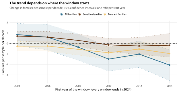
Three things fall out, and only the first is uncomfortable. Figure 8.2 is Table 8.6 with the three trends drawn against the start year, and each of the three is one of the shapes in it.
The headline magnitude is not a measurement, it is a choice. Across the 4 start years on which family counts are falling at all, the total runs from 0.34 to 2.06 families per sample per decade — a factor of 6.0. Start in 2004 or 2006 instead and the counts are still rising. So 1.49 is what this window says and not what the record says, and it should not be quoted without the window attached.
The tolerant decline is the stable part. It is negative under all 6 start years, from 0.25 to 0.96 families per sample per decade — a much narrower spread than the total, and the reason the ratio between them swings about is almost entirely the denominator. Stable is not the same as well determined, though: the interval is wholly below zero at 3 of the 6 starts (2008, 2010, 2014) and reaches above it at the other 3 (2004, 2006, 2012), which Table 8.6 sets out.
The recovery reading gets stronger, not weaker, as the window lengthens. Sensitive families never decline significantly under any start year, and on the two earliest windows they gain significantly (0.70 (0.25 to 1.15) from 2004, 0.60 (0.06 to 1.14) from 2006). The sensitivity is real, and it does not threaten the conclusion — it threatens the number.
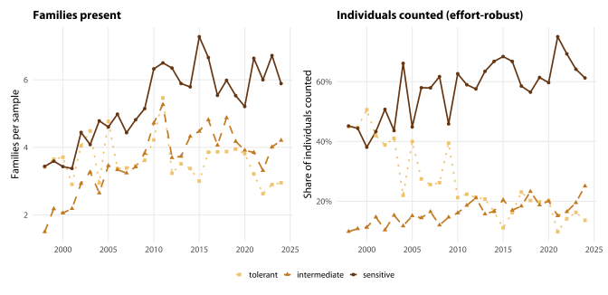
2 of the 117 families have no SIGNAL 2 grade and are excluded from the three sensitivity classes; they are retained in every other analysis.
8.6 Winners and losers
Two questions are asked of every family common enough to answer them: is it being found in a larger share of samples than it used to be (occupancy), and does it make up a larger share of the animals counted (relative abundance)? Families recorded in fewer than 20 of the 1,502 samples are excluded, because a trend cannot be estimated from a handful of records; 75 families remain.
Testing 75 families separately means 75 chances to find a spurious result. Chapter 6 has the cautionary version of that: an uncontrolled scan of site-level water quality trends flagged dozens of “significant” results, and once the false discovery rate was controlled over the whole family of tests the scan actually ran, not one of them survived. Both analyses here are corrected — the occupancy models by the Benjamini–Hochberg false discovery rate procedure (Benjamini and Hochberg 1995), the abundance models by mvabund’s own resampling-based adjustment, which is blocked on site here, so repeat visits to a creek are resampled together — a choice this analysis made, not a package default. mvabund fits a separate generalised linear model to each family and tests them jointly by resampling (Wang et al. 2012); it exists because a distance-based test on raw counts is dominated by the most abundant taxa — the mean-variance problem Warton et al. (2012) describe, and it is their result, not mvabund’s manual — and a per-family model with an explicit count distribution does not have that failure mode.
Four occupancy specifications are fitted and the strictest is the one reported: presence on decade, with sample size as a covariate and random intercepts for both site and year. The other three are printed so you can see what each correction costs, because the cost is large and a scan of this kind can be made to say almost anything.
| Specification | Increasing | Decreasing | Total of 75 |
|---|---|---|---|
| Time only, site random effect | 25 | 11 | 36 |
| Adding a year random effect | 19 | 3 | 22 |
| Adding sample size | 17 | 15 | 32 |
| Adding both (reported throughout) | 12 | 5 | 17 |
17 of 75 families changed in occupancy after false discovery rate control (12 up, 5 down). In relative abundance, mvabund flags 15 (6 up, 9 down); of the 10 families flagged by both, 10 move in the same direction.
Those two counts are not like for like, and the difference between them is mostly procedure rather than evidence: mvabund uses a step-down resampling adjustment that is much more conservative than Benjamini–Hochberg. Asking the abundance question the same way the occupancy question is asked — one negative binomial mixed model per family, the same offset, the same random effects for site and year, the same Benjamini–Hochberg correction — flags 24 families, 9 up and 15 down. The two sets of abundance coefficients correlate at 0.94, so this is a difference in how many results are declared, not in what the data say.
Not quite the same way for all of them. For 1 of the 75 the negative binomial would not converge. Empididae (dance fly) is recorded in 20 of the 1,502 samples, 21 animals in total, never more than 2 in a single sample. A count that is almost all zeros has no overdispersion in it for a negative binomial to measure, so the dispersion parameter runs off towards the Poisson limit, sits on the edge of its own parameter space, and leaves a Hessian that cannot be inverted for standard errors. glmmTMB says so, and declines to stand behind the fit. That family is refitted as the Poisson the dispersion parameter was heading for, which is the limiting case of the same model rather than a different question. It converges, and it moves the per-decade coefficient by 5.4e-06. The unconverged fit was not, in the end, pointing anywhere different — it simply could not say how sure it was. No family is left unfitted, so all 75 of those counts rest on a model that converged.
The two measures therefore disagree about the balance and agree about the direction. More families are spreading than retreating in occupancy (12 against 5), while more are falling than rising in relative abundance (15 against 9). Occupancy is this chapter’s effort-sensitive measure and relative abundance its effort-robust one, so the balance should be quoted from the abundance analysis. What both agree on is which families: the abundance trend rises with SIGNAL 2 at 0.151 per grade (p = 2.5e-05), so the families losing ground in abundance are the tolerant ones.
| Family | Common name | Odds per decade | SIGNAL 2 | SIGNAL-SF | EPT | Samples |
|---|---|---|---|---|---|---|
| Tasimiidae | caddisfly | 4.54 | 8 | 8 | yes | 75 |
| Gripopterygidae | stonefly | 4.06 | 8 | 9 | yes | 846 |
| Leptoceridae | long-horned caddisfly | 2.53 | 6 | 8 | yes | 1338 |
| Philorheithridae | caddisfly | 2.44 | 8 | 9 | yes | 349 |
| Helicopsychidae | snail-case caddisfly | 2.28 | 8 | 10 | yes | 135 |
| Hydroptilidae | micro-caddisfly | 2.04 | 4 | 6 | yes | 465 |
| Simuliidae | blackfly larva | 1.92 | 5 | 4 | – | 383 |
| Baetidae | small minnow mayfly | 1.86 | 5 | 6 | yes | 530 |
| Scirtidae | marsh beetle | 1.68 | 6 | 8 | – | 486 |
| Ceratopogonidae | biting midge | 1.55 | 4 | 6 | – | 641 |
| Tipulidae | crane fly | 1.47 | 5 | 7 | – | 507 |
| Elmidae | riffle beetle | 1.45 | 7 | 7 | – | 425 |
| Family | Common name | Odds per decade | SIGNAL 2 | SIGNAL-SF | EPT | Samples |
|---|---|---|---|---|---|---|
| Culicidae | mosquito larva | 0.25 | 1 | 6 | – | 200 |
| Veliidae | small water strider | 0.43 | 3 | 7 | – | 1248 |
| Synlestidae | damselfly | 0.49 | 7 | 7 | – | 260 |
| Dytiscidae | diving beetle | 0.56 | 2 | 7 | – | 671 |
| Notonemouridae | stonefly | 0.58 | 6 | 8 | yes | 157 |
Two families that look like losers on a weaker model are deliberately absent from Table 8.9. Oniscidae (slater) and Talitridae (landhopper) are terrestrial and semi-terrestrial animals that turn up in an edge sweep as bank strays rather than as members of the aquatic assemblage. They are recorded in 21 and 21 samples respectively — one above the inclusion floor of 20 — they carry the two largest standard errors in the whole set of 75, and neither survives the specification used here. A change in whether a sorter bothers to record a woodlouse is a more parsimonious explanation of their apparent decline than an ecological one. Nothing in either database records identification practice, so we cannot check it — which is why it is a question for you rather than a finding (dq:terrestrial-taxa-convention).
| Group | Families | Mean SIGNAL 2 | Mean SIGNAL-SF | EPT families |
|---|---|---|---|---|
| Increasing in occupancy | 12 | 6.2 | 7.3 | 7 of 12 |
| Decreasing in occupancy | 5 | 3.8 | 7.0 | 1 of 5 |
| No detectable change | 58 | 4.8 | 6.1 | 15 of 58 |
The families gaining ground are the sensitive ones. Families increasing in occupancy average SIGNAL 2 6.2; families decreasing average 3.8. 7 of the 12 increasing families are mayflies, stoneflies or caddisflies — the pollution-sensitive orders on which the health rating’s EPT factors are built — against 1 of the 5 decreasing families.
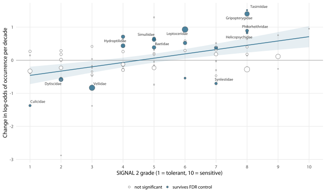
Table 8.10 compares two groups defined by their own p-values, and with 5 families in the decreasing group it cannot carry a formal test. The relationship is better put continuously, across all 75 families tested: the occupancy trend rises by 0.130 in log-odds per decade for every SIGNAL 2 grade (p = 2.2e-05), explaining 22% of the variation between families. That is the recovery signal stated as a slope rather than as a count, it uses every family rather than the ones that crossed a threshold, and it is what Figure 8.4 draws.
Effort sensitivity of this section. Occupancy is the one headline measure here that could in principle be inflated by larger samples: a family present at low density is more likely to be detected when more animals are picked. That is why sample size is in the model rather than beside it. Its effect on the estimates is modest — adding it shrinks them by a median of 11% and reverses the direction of 0 of them — but its effect on how many results are declared is not, and Table 8.7 is the honest accounting: 36 families under the weakest specification, 17 under the strictest. The abundance analysis is effort-proof by construction, because sample size enters it as an offset, and it points the same way about which families are gaining. The individual odds ratios below are still best read as upper bounds.
One result deserves comment because it cuts against the general pattern. Notonemouridae (stonefly) is a sensitive stonefly, and Synlestidae (damselfly) a sensitive damselfly, yet both are becoming less widespread. Neither overturns the overall picture — the slope across all 75 families runs firmly the other way — but they are a reminder that “tolerant” and “sensitive” are summaries of a family’s typical behaviour, not a prediction for any single creek.
8.6.1 The thing your rating cannot see
This one is about the index rather than about the creeks, and it decides what the rating can report.
The recovery is a shift along the sensitivity scale. So the obvious question is whether the scale in the health rating — SIGNAL-SF — can see it. Run the same continuous comparison as above on SIGNAL-SF instead of SIGNAL 2 and it is a real but much weaker predictor of which families are spreading: slope 0.077 per grade (p = 0.039), explaining 5.7% of the between-family variation against SIGNAL 2’s 22%. Put both scales in one model and SIGNAL 2 keeps its coefficient (0.159, p = 1.2e-04) while SIGNAL-SF’s falls to -0.049 (p = 0.28). The two correlate at 0.68 across the 75 families tested, so these are not two measures of different things: the scale in your rating is a noisier version of one that works.
The mechanism is visible in Table 8.8 and Table 8.9. SIGNAL-SF gives 6 to the mosquito Culicidae (mosquito larva) and 7 to the diving beetle Dytiscidae (diving beetle) and the water strider Veliidae (small water strider), where SIGNAL 2 gives 1, 2 and 3. The families that are disappearing are graded as though they were clean-water animals, so their disappearance barely moves the average.
And there is a second, deeper reason, which is about what SIGNAL-SF omits rather than how it grades. SIGNAL-SF has no grade at all for exactly the taxa that dominate a degraded sample — oligochaete worms, chironomids identified no further than family, mites. Those animals are invisible to SIGNAL-SF and fully counted by SIGNAL 2. An assemblage shifting from tolerant worms and midges towards sensitive insects therefore moves SIGNAL 2 a long way and SIGNAL-SF barely at all.
Put the two facts side by side. The largest, most robust signal in the whole monitoring record is a shift from tolerant families to sensitive ones — and the index your rating is built on is, by construction, the one least able to register it. That is not a small calibration issue. It means the rating has been reporting a creek network that is recovering as one that is roughly static.
You might want to test SIGNAL 2 as a replacement factor. It is the current national version of the index, with grades re-derived across Australian regions from field data rather than carried over from the original expert assignment (Chessman 2003); the earlier objective derivation (Chessman et al. 1997) was for the Hunter River system and its authors warned it might not generalise. It also grades the coarse taxa SIGNAL-SF leaves out. Chapter 15 is where that gets tried.
Chapter 5 has the same result seen from the other end: on the health score itself, SIGNAL-SF moves about a quarter as far as SIGNAL 2 over the record, and the share of individuals carrying no SIGNAL-SF grade — which drifts over time — is not what is driving the gap.
8.7 Are the creeks becoming more alike?
Urbanisation usually makes streams resemble one another: tolerant, widespread animals replace the local specialists, and creeks that were once distinctive converge on the same short list of survivors. Ecologists call it biotic homogenisation (Olden and Rooney 2006), and urbanisation is McKinney (2006)’s “one of the most homogenizing of all major human activities” — he reviews plants, birds, mammals and insects and finds urban assemblages converging worldwide.
It is worth testing here for one specific reason: it would be invisible to every metric you currently report. Every creek could hold the same number of families, at the same average sensitivity, while the network as a whole lost what made its creeks different from each other.
The test averages each creek’s samples within a year, then measures how different those creek-averages are from one another, year by year.
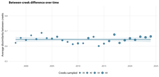
No detectable homogenisation, bounded at 6.4% of the observed level. Average between-creek dissimilarity changes by 0.000 per decade (95% CI -0.011 to 0.011), over 27 annual points covering 26 years of the macroinvertebrate record. The analysis can detect a change of 0.016 Bray–Curtis units per decade at 80% power — 0.04 across the record, or 6.4% of the observed level of 0.64.
Read that as a bound, not as an absence. A homogenisation that large or larger is ruled out; a smaller one is not, and nothing here shows there is none. What can be said is that Blue Mountains creeks have kept their individual identities as far as these data can see — which is not something that could have been assumed, because urbanisation is the most consistently reported driver of homogenisation there is and these are urbanising catchments.
Where that bound comes from, and why the textbook version of it is too small here. The standard closed form for a two-sided test at 80% power is written with normal quantiles, and on this series that is the wrong reference distribution: there are 27 annual points, so the slope test carries 25 residual degrees of freedom, not infinitely many. Taking the quantiles from that t distribution instead is the difference between 0.015 per decade and the 0.016 published above — about 4.1% larger, and it matters because the smaller figure does not do what a minimum detectable effect is for. Its real power is 77%, not 80%. The t bound’s is 80%, and 2,000 datasets simulated from the fitted model with exactly that slope recover a rejection rate agreeing with it to within 0.3 percentage points — the closed form and the fitted model agree, which is the check that would have caught an error in either, and did. Chapter 19 quotes 6.4%, this figure.
The number of creeks sampled changes from year to year — 24 to 66 — and adding a distinctive creek raises the average dissimilarity by itself, so the all-creek series alone would not settle this. The direct comparison does. Take the 38 creeks with samples in both 1998–2006 and 2016–2024, average each creek within each window, and measure dissimilarity among the same 38 creeks in each: 0.570 early against 0.548 late, a change of -0.022 with a creek-bootstrap 95% interval of -0.074 to 0.030. No creek enters or leaves between the two numbers being compared.
Two readings of that are available and the data do not separate them. Either these catchments are not urbanising fast enough, or from a low enough base, for convergence to have begun — the record starts in 1998, in suburbs that were already built, so the largest losses may predate it. Or the differences between these creeks are set by things urbanisation does not touch: altitude, position in the network, catchment area, which chapter 9 finds to be the dominant axes. Either way the practical consequence is the same and it is a good one — the network still contains distinguishable creeks, and protecting them individually is still worth doing.
Section 8.4.2 answers the related question, whether individual samples are becoming more variable, and reaches the same conclusion.
Effort sensitivity of this section. None. Every quantity here is a Bray–Curtis dissimilarity between relative abundances of creek-year averages. A creek whose samples were processed more thoroughly contributes the same proportions.
8.8 What is the change associated with?
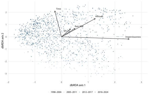
Composition responds to many things at once. Variance partitioning asks how much of the difference between communities each broad category of explanation can claim: time, catchment condition (total catchment imperviousness), space (altitude and which major catchment the creek sits in), and climate (antecedent rainfall over 90 days and 12 months, and the 12-month standardised precipitation index). Because the categories overlap, the analysis reports what each explains uniquely, after the other three have taken what they can.
For management this is the most useful output in the chapter, because it separates what you can change from what you cannot.
Chapter 9 refits this same partition with two more blocks in it — same method, same response, water quality and physical habitat added — so the percentages there are not the percentages here and the two are not in disagreement. If you want the driver ranking, take chapter 9’s: it is the better model and this one is the four-block special case of it. What is here is what this chapter needs in order to say that the compositional change is not mostly the calendar.
| Component | Share of community variation |
|---|---|
| Time | 3.0% |
| Catchment imperviousness | 4.3% |
| Space (altitude, catchment) | 3.3% |
| Climate | 1.5% |
| Shared between components | 4.2% |
| Explained in total | 16% |
| Unexplained | 84% |
Three things follow.
- Catchment condition and geography together outweigh time. Imperviousness uniquely explains 4.3% and space 3.3%, against 3.0% for time — so where a creek is and what its catchment is like account for about 2.5 times what 26 years of change account for.
- Climate is real but minor. Antecedent rainfall and drought index uniquely explain 1.5%. Chapter 5 reached the same conclusion for the health score: the improvement is not the drought breaking.
- Most variation is unexplained, at 84%. Sample-level macroinvertebrate data are noisy: which animals end up in a net on a given morning depends on things no monitoring program records. This is not a failure of the model, and the components above are estimated well despite it.
These percentages are upper bounds, and the ratios between them are the trustworthy part. Bray–Curtis distances are not Euclidean, so the ordination has imaginary axes as well as real ones, and the negative eigenvalues shrink the denominator every adjusted R-squared here is divided by. Chapter 9 quantifies it on its own six-block partition (Section 9.4.2): about a quarter of the eigenvalue mass there is negative, and on a metric embedding magnitudes like those in Table 8.11 roughly halve. The ordering of the blocks does not change, and neither does the conclusion. If you quote a percentage from this section, quote Section 9.4.2’s corrected version with it.
Effort sensitivity of this section. Low, but not nil. The response is Bray–Curtis dissimilarity between relative abundances, so it is effort-robust, but sampling effort is not one of the four blocks and it is correlated with time. The time fraction of 3.0% is therefore an upper bound: the within-site PERMANOVA in Section 8.4.1, which does fit effort explicitly and before time, is the specification to prefer where the two differ.
| Term | df | Pseudo-F | p |
|---|---|---|---|
| Time (decades) | 1 | 55.1 | < 0.005 |
| Catchment imperviousness | 1 | 96.0 | < 0.005 |
| Altitude (m) | 1 | 42.0 | < 0.005 |
| Rainfall, previous 90 days | 1 | 7.0 | < 0.005 |
| 12-month drought index (SPI-12) | 1 | 10.2 | < 0.005 |
Two of those five terms — imperviousness and altitude — do not vary within a creek, so testing them against the residual degrees of freedom of 1,319 samples credits them with far more information than the design holds. Repeating the test on one averaged community per creek gives the honest version, and both survive it: imperviousness F = 12.5, p = 0.001, and altitude F = 5.8, p = 0.001, on 90 creeks with 999 permutations. The directions in the biplot in Figure 8.6 are therefore real; the p-values in Table 8.12 are not to be read as evidence about how strong they are.
8.9 A field-guide version of this
The families that most reliably mark a good site and a poor one — the ones worth knowing by sight on a bank — are set out in Section 8.10 below, with common name and sensitivity grade. It is the one table out of this chapter a field officer would actually carry.
8.10 Indicator families
An indicator analysis asks a simpler and more practical question than a trend: which families, if you found them, would tell you most about where you were? This is directly useful for field staff and for public communication. The statistic is the indicator value of Dufrêne and Legendre (1997), which multiplies how faithful a family is to one group of sites by how often it is found there, so that a family scores highly only if it is both largely confined to the group and reliably present in it; the permutation test and the several variants of the index are those of De Cáceres and Legendre (2009).
Catchment disturbance tier is a property of the creek, not of the sample. A creek visited forty times supplies forty copies of the same tier label, and an indicator analysis run over all 1,502 samples with free permutation treats those forty as forty independent pieces of evidence. That is the same error Section 8.4.1 builds a separate between-site design to avoid, so the tier analysis is run the same way: one averaged community per creek, 125 rows rather than 1,502. Era does vary within a creek, so the era analysis keeps every sample, with permutations restricted to stay within a creek.
| Catchment tier | Family | Common name | Indicator strength | SIGNAL 2 |
|---|---|---|---|---|
| Reference | Notonectidae | backswimmer | 0.75 | 1 |
| Reference | Leptophlebiidae | prong-gilled mayfly | 0.68 | 8 |
| Slightly disturbed | Baetidae | small minnow mayfly | 0.80 | 5 |
| Slightly disturbed | Philorheithridae | caddisfly | 0.71 | 8 |
| Slightly disturbed | Leptoceridae | long-horned caddisfly | 0.69 | 6 |
| Slightly disturbed | Philopotamidae | finger-net caddisfly | 0.66 | 8 |
| Slightly disturbed | Odontoceridae | caddisfly | 0.61 | 7 |
| Slightly disturbed | Calocidae | caddisfly | 0.50 | 9 |
| Slightly disturbed | Atriplectididae | caddisfly | 0.44 | 7 |
| Urban | Veliidae | small water strider | 0.73 | 3 |
| Era | Family | Common name | Indicator strength | SIGNAL 2 |
|---|---|---|---|---|
| 1998–2004 | Veliidae | small water strider | 0.63 | 3 |
| 1998–2004 | Dytiscidae | diving beetle | 0.53 | 2 |
| 1998–2004 | Synthemistidae | tigertail dragonfly | 0.45 | 2 |
| 1998–2004 | Culicidae | mosquito larva | 0.40 | 1 |
| 2005–2011 | Megapodagrionidae | damselfly | 0.42 | 5 |
| 2005–2011 | Dugesiidae | flatworm | 0.38 | 2 |
| 2005–2011 | Parastacidae | freshwater crayfish (yabby) | 0.34 | 4 |
| 2005–2011 | Synlestidae | damselfly | 0.30 | 7 |
| 2012–2017 | Hydroptilidae | micro-caddisfly | 0.44 | 4 |
| 2012–2017 | Simuliidae | blackfly larva | 0.41 | 5 |
| 2012–2017 | Ecnomidae | caddisfly | 0.31 | 4 |
| 2012–2017 | Physidae | bladder snail | 0.27 | 1 |
| 2018–2024 | Leptoceridae | long-horned caddisfly | 0.54 | 6 |
| 2018–2024 | Gripopterygidae | stonefly | 0.54 | 8 |
| 2018–2024 | Ceratopogonidae | biting midge | 0.49 | 4 |
| 2018–2024 | Baetidae | small minnow mayfly | 0.44 | 5 |
Table 8.13 is short, and that is the point of running it at the honest sample size. At the sample level 10 families would have become several dozen, most of them riding on creeks that happen to have been visited often. What survives is a handful of families that genuinely distinguish one class of catchment from another.
One entry deserves a caution. Notonectidae (backswimmer) appears as a reference indicator despite a SIGNAL 2 grade of 1, because indicator analysis reflects habitat as well as condition: several reference sites are upland swamps and pools where backswimmers are naturally abundant. Indicator families identify where you are, not how healthy it is, and the two are not the same question.
Table 8.14 is this chapter in miniature. The families that best mark the earliest years are Veliidae (small water strider) and Dytiscidae (diving beetle), both tolerant; the families that best mark the most recent years are Leptoceridae (long-horned caddisfly) and Gripopterygidae (stonefly), both sensitive EPT families.
8.11 What this chapter will and will not bear
It will bear the direction, and it will not bear any single family. The tolerant-to-sensitive shift is a slope across all 75 families tested, not a count of families that crossed a threshold, and it survives a year random effect, a sample-size term and rarefaction to a constant number of individuals. An individual odds ratio in Section 8.6 is a much weaker thing: occupancy carries a residual detection component, so read those as upper bounds.
Every model here carries a year random effect, and that is not cosmetic. Samples taken in the same year share the weather, the crew, the sorting bench and that year’s identification conventions. Putting a year term in withdraws the whole-record tolerant richness decline, the post-2010 intermediate decline, and 14 of the per-family occupancy results that a site-only model would have declared — 19 once the sample-size term goes in beside it, which is the specification reported throughout (Table 8.7). What survives is in Section 8.5 and Section 8.6.
Association, not causation. Creeks with high imperviousness differ from creeks with low imperviousness in many ways beyond imperviousness, and the passage of time is a proxy for everything that changed over 26 years — including your own works programs, which are not recorded in a form that can be analysed. Chapter 17 is where the design for actually testing a works effect lives.
The variance partition describes the modern network, not the whole record. A recorded altitude is not available for all legacy sites and is the binding constraint on this set: Section 8.8 is fitted on 1,319 of the 1,502 samples, from 90 of the 125 creeks that have a modelled catchment, recorded altitude and complete climate covariates. Imperviousness is modelled and is available for 117 of the 125 creeks.
Everything else — what the analysis set is, what it excludes and why, and the questions only you can settle — is in the data section at the head of the chapter.
| Item | Value |
|---|---|
| Data layer built | 2026-08-30 12:56 |
| R version | R version 4.4.3 (2025-02-28) |
| Primary analysis set | 1,502 edge stream samples, 125 sites, 1998-2024 (26 years of the macroinvertebrate record), 117 families |
| Family count used | Strict (family-level, microfauna dropped) — not the published n_families |
| Families tested individually | 75 of 117 (recorded in 20 or more samples) |
| Model fits | read from the targets graph in R/_targets.R |