| Parameter | n | Exactly zero | Publish a pass rate? | Why |
|---|---|---|---|---|
| Alkalinity (ppm CaCO3) | 1,139 | 0.3% | Yes | laboratory, off the probe, 0.3% zeros; check the 1998-99 placeholders first |
| Conductivity (µS/cm) | 1,128 | 0% | Yes, within altitude zone and probe era | failure rate steady across probes (1.5-fold), no zeros; but the level steps at both probe changes (Section 6.9), so score within an era; the range differs by altitude zone |
| Nitrate-N (ppm) | 948 | 4.5% | Yes | laboratory, range starts at 0.04 so non-detects score below, not within; from 2006 |
| Phosphate (ppm, as PO4 or as P) | 1,044 | 54% | No — report detectability instead | 70% of its passes are exactly zero; the range starts at 0 |
| Dissolved oxygen (mg/L) | 1,253 | 0% | Not yet — rebaseline first | failure rate moves 6.7-fold across the three probes |
| Dissolved oxygen (% sat.) | 1,170 | 0% | No — use mg/L | the same measurement as mg/L; failure rate moves 3.8-fold between probes |
| Faecal coliforms (CFU/100mL) | 941 | 37% | Detectability only, from 2006 | 57% of passes are exactly zero, against a confirmed limit of 10 CFU/100 mL |
| pH | 1,293 | 0% | Not yet — rebaseline first | failure rate moves 2.0-fold across the three probes |
| Salinity (PSU) | 1,075 | 0% | No — use conductivity | pre-2020 values sit on a 0.01 PSU grid and the higher-zone range is 0.01 PSU wide — one grid step |
| Turbidity (NTU) | 1,187 | 21% | No — report nothing | both problems at once: 33% of passes are zeros, and the failure rate moves 3.3-fold between probes |
7 The water quality report card
Blue Mountains City Council Healthy Waterways — statistical analysis
7.1 What this chapter is for
Chapter 6 asks what changed in the water quality record. This chapter asks the narrower question you actually have to answer when someone wants a figure for a newsletter, a council report or a web page: of the numbers this record can produce, which ones may be printed?
It is mostly a chapter about what may not be. That is not an enthusiastic thing to write, so it is worth saying at the top that every refusal below comes with an alternative — a different statistic that says something true about the same parameter — and that three of the ten parameters come through publishable, though not all three unconditionally. Table 7.1 is the whole answer, conditions included.
7.2 The data behind this chapter
Each question and request below is set out again in What we need from you, with what it blocks, what an answer is worth and what it would cost you to find, ranked against every other ask in the report.
7.2.1 Questions only you can answer
The share of turbidity readings above the 7.08 NTU trigger falls by a factor of three across the three probes, and dissolved oxygen moves nearly seven-fold the other way. Would you rather we left both out of the report card, or published them with the instrument era printed beside them?
Each probe reads systematically lower than the last, and a probe that reads lower crosses a fixed threshold less often. Chapter 3’s verdict table (Table 3.1) records the turbidity change as not separable from the method. Conductivity is the counter-example that makes the rule usable — it moves 1.5-fold across the same three instruments, which is what a stable measurement looks like.
Refer to it as
dq:exceedance-tracks-the-probe.
When phosphate is written down in ppm, is that phosphate as PO4 or as phosphorus? The kit’s instruction sheet, a results header or whoever set up the spreadsheet would settle it.
The field is AvailPhosphate and the unit is ppm, and nothing in either database, in the field sheets or in the methods document says which of the two conventions the number follows. They differ by a factor of 3.07, so a reading of 0.03 ppm is either 0.03 ppm of phosphorus or about 0.01 ppm of phosphorus depending on which was meant. Your nitrogen field says which it is — it is called Nitrate-Nitrogen — and the phosphate field does not. Your own 2024 desirable ranges are safe either way, because they were derived from percentiles of these same readings, so both sides of a pass or a fail carry whatever convention the kit used and it cancels. What is not safe is any number that leaves the building.
Refer to it as
dq:phosphate-units.
For phosphate, turbidity and faecal coliforms the desirable range starts at zero, so a reading the test could not see is scored as a pass. Are you happy for us to print the non-detect rate beside those three wherever the pass rate appears?
It is not a small correction. 70% of phosphate’s “within the desirable range” flags in the analysis set are stored as literal zeros — 71% if you also count the readings below the inferred 0.01 ppm limit, and the chapter keeps those two figures apart because only one of them needs a limit nobody has confirmed. Not one of the 247 “above” flags is a zero. For faecal coliforms, whose detection limit of 10 CFU/100 mL is the one that is actually confirmed, 73% of the passes are below that limit. Printing the pass rate on its own reports the test kit. Printing both numbers is honest and costs one extra column.
Refer to it as
dq:zero-start-ranges.
What, if anything, do you want the public report card to say about phosphate? Our suggestion is to report detectability, label it plainly as a property of the test, and not score it.
Publishing “phosphate met the desirable range in 89% of measurements” — the figure for the 2022-2024 report-card window; over the whole record it is 76% — would report the test kit, not the creek, because most of those measurements are non-detects scored as passes. Detectability is defensible as reporting and is not defensible as scoring. There is reputational risk either way — saying nothing invites the question, and saying the wrong thing is worse — so this one should be a decision you take deliberately.
Refer to it as
dq:phosphate-reportcard-decision.
Are you happy for us to keep site-level water quality out of the report card until the sampling calendar and the instrument changes are dealt with? It is the least welcome finding in the chapter and we would rather you decided it than discovered it.
The site-level scan runs 648 site-by-parameter tests and not one survives false discovery rate control, so no creek in the network can be singled out on this evidence. We know officers use site-level water quality to direct field effort, which is exactly why this needs saying out loud rather than by omission. It is fixable — a stable sampling calendar, probe overlap at each changeover, and a defined core set of sites on a fixed schedule would make the question answerable.
Refer to it as
dq:site-level-reporting-decision.
How were bounded and estimated plate counts recorded? Three of the largest values in the record went in as “>10,000”, “TNTC” and a conservative estimate entered as though it were measured.
23,000 is the fourth-largest post-break coliform value and it is not a measurement — the field note estimated it “conservatively as this is the highest recorded”, and it was not: the same site had already read 29,000 thirteen months earlier, and 182,000 there in 2017 and 88,500 at 86BKT in 2022 are both larger again. Any coliform maximum or mean published from this record leans on those three numbers, so the convention matters more than the count of affected rows suggests.
Refer to it as
dq:coliform-bound-convention.
Should the report card be built from the macroinvertebrate program’s stream samples, from every stream water quality sample including the recreational program, or from both reported separately?
Both are defensible and they give different answers. On 2022–2024 stream samples the pH pass rate is 67% on the macroinvertebrate program and 49% on all stream samples — a 17-point gap on the same period, the same waterbody type and the same published ranges. The recreational program samples swimming holes rather than the monitoring network, so the two sets genuinely differ. Whichever you choose, the report card has to say which, or it has published an ambiguous number.
Refer to it as
dq:report-card-sample-set.
Would you like us to switch replicate coliform averaging from an arithmetic to a geometric mean, as ANZECC/ARMCANZ specifies?
It affects sixteen sample codes, so it is small. But the current choice is indefensible if anyone asks, and changing it moves numbers you have already published — which is why it should be your call rather than ours.
Refer to it as
dq:coliform-mean-decision.
7.2.2 What would answer them
Can you find anything that names the phosphate test kit or reagent used between 2002 and 2024, and states what it can detect — a purchase order, an invoice, a stores ledger entry, even a photograph of a kit box? One dated point would help; two or three would settle it.
This is the same ask as chapter 3’s lab-detection-limits, narrowed to the one parameter it would unblock fastest — and it is not quite as small as it once looked. The floor did not move during the record, so there is one limit to confirm rather than a dated history of two kits: the smallest positive phosphate reading is 0.010 ppm in every year including 2012, and the seven readings that sit at 0.005 are averages of two replicates reading 0.00 and 0.01 rather than values the kit ever reported. But that only shows us the grid the results were written on, which is not the same thing as what the kit could see — a kit with a 0.1 ppm floor writing onto a 0.01 grid would leave exactly this trace, and one 2008 field note reading “Phos <0.1” suggests it might have. With an answer, phosphate becomes the strongest candidate in the set; without it, the 89% of the 2022-2024 report-card window’s phosphate measurements that sit inside the desirable range is mostly a statement about the kit.
Refer to it as
dq:phosphate-kit-history.
Is there a working spreadsheet or method note behind the 2024 desirable ranges — which sites, which years, and which instrument each reading came off? We have reconstructed them as 20th–80th percentiles of reference and slightly disturbed sites, 2006–2023, and we would like to check that.
Everything this chapter prints is a comparison against those ranges, so their derivation decides what the numbers mean. Two things we would want to see in it. The dissolved oxygen and turbidity ranges pool the Hydrolab and Aquaread eras, so the published range for those two describes a mixture of two instruments and every future pass rate is measured against the mixture. And the site list is 32 stream sites and two wetlands, so the published ranges are a stream distribution with a token of wetland in it rather than a wetland benchmark — which is why wetland readings are excluded here (chapter 11).
Refer to it as
dq:desirable-range-derivation.
7.3 What may be printed, and what may not
Ten of the eleven parameters have a published desirable range; water temperature has none, so there is no pass or fail to print for it at all. Here is the whole answer in Table 7.1, and the rest of the chapter is why.
Four rules fall out of it, and they are the practical content of this chapter.
- Report per parameter, never pooled. A pooled “% within the desirable range” is dominated by whichever parameters happen to have been measured most, which is a decision about field kit rather than about water. The pool in this record is two thirds probe parameters.
- Print the share of readings that are exactly zero beside any parameter whose desirable range starts at zero. There are three of them — phosphate, faecal coliforms, turbidity — and for all of them a “pass” and a “non-detection” are literally the same event.
- Do not publish an exceedance rate that moves with the probe. Turbidity’s moves 3.3-fold across the three instruments and dissolved oxygen’s 6.7-fold, neither of which is a creek changing.
- Say which samples the number counts. There are two defensible ways to say “stream samples” here, and for one parameter the 2022–2024 pass rate moves by more than ten percentage points between them. Nothing on a report card says which was used. Section 7.8 works it through.
Three parameters come through publishable — alkalinity, conductivity and nitrate-N. Conductivity does not come through unconditionally, though: it may be published only within altitude zone and probe era. They are the same three chapter 6 finds fit to enter a health rating (Section 6.9), which is reassuring but not a coincidence: both lists are mostly asking whether the measurement survived the changes in method.
7.4 Exceedance of the desirable ranges
Before any of the refusals above can be argued, the pass-or-fail machinery has to be on the table. The desirable ranges published in the 2024 revision turn each measurement into a pass or a fail, which is the most management-legible thing this dataset supports — and the question a report card asks of them is whether the failure rate has moved. It has. This section is how much, and it is the evidence the four rules rest on.
The published ranges are for streams. 2,500 of the 15,633 comparisons in wq_trigger_flags are wetland samples scored against a range derived from a site list of 32 stream sites and two wetlands — a stream distribution with a token of wetland in it, not a wetland benchmark. Every row in this chapter carries trigger_applicable == TRUE, so none of them is here. Leaving them in would move the headline “% above the desirable range” by three to seven points on four parameters and much more within the wetland subgroup — chapter 11 sets that out at Section 11.5, and it also flags one lake site currently classified as a stream.
7.4.1 The record as a whole
Figure 7.1 is the whole record in one picture, and the rest of this section is what can and cannot be read off it.
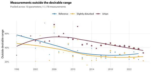
Pooled across parameters and sites, the odds of a measurement falling outside its desirable range fall by a factor of 0.71 per decade (95% CI 0.59 to 0.84; 11,178 comparisons, 122 sites, 10 parameters) — about a 29% reduction in the odds of a failure per decade. Urban sites fail 1.68 times as often as reference sites (1.24 to 2.28).
Read “failure” narrowly. The outcome is outside the range in either direction, and 22% of these failures are readings that fell below the desirable range rather than above it — which for several parameters is cleaner water, not dirtier (Section 7.4.4 sets out which, and on what basis). So this is a movement towards the middle of the range, not a measured fall in pollution. Both splits are published: Section 7.4.4 gives it for the exceedance count, and Table 7.4 gives it for the exceedance trend — count only the above-range readings as a failure and the same model returns 0.85 per decade (0.68 to 1.06), an interval that includes 1. A reader who takes the number above to mean “29% fewer pollution exceedances per decade” has read more into it than it says.
That pooled figure is here because it is the one the modelling supports; rule 1 above says do not print it, and the two statements are compatible — a number can be the right summary for a chapter and the wrong summary for a report card.
This is the common slope, from a model with a single time term. A second model, fitted only to test whether the tiers differ, adds a time-by-tier interaction; its interaction terms are 1.04 for urban against reference (0.82 to 1.32) and 1.08 for slightly disturbed (0.84 to 1.40).
The three tiers improve at rates that are statistically indistinguishable, so there is no evidence that the gap between urban and reference catchments is closing. Read the interval rather than the verdict, though: with only 16 reference sites in this chapter’s stream-only trigger set — Section 12.3 enumerates the several populations this book calls reference, and they differ in size, so the bare phrase is never enough on its own — the urban-against-reference term runs from 0.82 to 1.32 per decade, so a gap that was closing, or widening, by a good deal would still have come back as “no difference”. This is an absence of evidence, not evidence of sameness. Chapter 5 reaches the same place for macroinvertebrate health with far more data.
One more thing a report card needs to know: whether the improvement is still going on, or whether it happened early and stopped. Splitting the record at the changepoint chapter 5 estimates for waterway health (Section 5.5.2) — the changepoint year itself going to the later window, which is where chapter 5 puts it in its own split, so the two windows partition the 11,178 measurements fitted here rather than sharing any — gives 0.92 per decade before (0.56 to 1.51, n = 4,130) and 0.78 after (0.64 to 0.96, n = 7,048), and a change-of-slope term at 2014 is not supported (p = 0.67). The first window is too thin to say much on its own — its interval runs from a 44% fall to a 51% rise in the odds per decade, so it is consistent with almost anything — but nothing here says the improvement stopped, so comparing this year’s pass rate with 2015’s is not obviously unfair. The change-of-slope test beside it is the better instrument for the same question: it is fitted on the whole record with a hinge term rather than on two windows, so it neither loses power to the split nor depends on which side of it the changepoint year is counted.
7.4.2 By parameter
| Parameter | n | % outside | % exactly zero | Odds ratio per decade | Survives era test? |
|---|---|---|---|---|---|
| Turbidity (NTU) | 1,187 | 37% | 21% | 0.18 (0.07 to 0.48) | Yes |
| Phosphate (ppm, as PO4 or as P) | 1,044 | 24% | 54% | 0.42 (0.17 to 1.03) | n/a — no change |
| Dissolved oxygen (mg/L) | 1,253 | 36% | 0% | 0.49 (0.33 to 0.74) | Yes |
| Alkalinity (ppm CaCO3) | 1,139 | 42% | 0.3% | 0.55 (0.32 to 0.94) | Weakened |
| Dissolved oxygen (% sat.) | 1,170 | 40% | 0% | 0.67 (0.42 to 1.07) | n/a — no change |
| pH | 1,293 | 45% | 0% | 0.71 (0.38 to 1.32) | n/a — no change |
| Faecal coliforms (CFU/100mL) | 941 | 35% | 37% | 0.72 (0.45 to 1.16) | n/a — no change |
| Nitrate-N (ppm) | 948 | 60% | 4.5% | 0.76 (0.43 to 1.34) | n/a — no change |
| Conductivity (µS/cm) | 1,128 | 44% | 0% | 0.83 (0.55 to 1.26) | n/a — no change |
| Salinity (PSU) | 1,075 | 48% | 0% | 1.66 (1.07 to 2.58) | No — sign flips |
The improvement is broad — nine of the ten parameters with a desirable range move in the right direction (Table 7.2) — but it is not evenly distributed. Turbidity carries much the steepest decline (odds ratio 0.18), and it is the parameter whose measurement is least trustworthy. Phosphate is next (0.42), and Section 7.5 shows what that number is really measuring. Faecal coliforms, once the series is started at 2006 rather than across the break, are unremarkable (0.72); carry the pre-break readings in and they become one of the two steepest declines in the set, which is the break talking and not the creeks. Salinity is the single parameter moving the wrong way (1.66), which is the conversion artefact chapter 6 sets out at Section 6.9: the probe changed what it reports as salinity, and salinity is the only parameter here moving the wrong way because of it.
So: how much of the pooled improvement do the measurement-affected parameters carry? Refitting the pooled model with them removed, always in the same form:
| Model | Measurements | Odds ratio per decade | Adjusted for probe era |
|---|---|---|---|
| All ten parameters | 11,178 | 0.71 (0.59 to 0.84) | 0.69 (0.52 to 0.93) |
| Minus turbidity and faecal coliforms | 9,050 | 0.72 (0.60 to 0.87) | 0.63 (0.46 to 0.85) |
| … also minus phosphate | 8,006 | 0.75 (0.63 to 0.89) | 0.67 (0.50 to 0.90) |
| … also minus salinity | 6,931 | 0.72 (0.59 to 0.87) | 0.70 (0.51 to 0.98) |
The improvement survives removing every parameter with a known measurement problem. It is the single most defensible result in this chapter.
Adding an instrument-era term to each of the models in Table 7.3 — the confound Section 7.4.3 describes, which no pooled model in this chapter carried until now — widens every interval by about 71% and leaves all four still separable from 1. The row that comes closest is … also minus salinity, whose upper limit is 0.98. So the improvement is not an artefact of the probe replacements: it survives adjusting for them, on the same two-sided ranges used throughout. What the era term costs is precision, not the direction — the era and time terms are nearly collinear, for the reason set out in Section 7.4.3, so the adjusted fit is a weaker instrument rather than a contradicting one.
How much of it turbidity and faecal coliforms account for is not well determined: the answer is 7% with year-level clustering modelled and 23% without it. The defensible statement is that the pooled odds ratio moves from about 0.71 to about 0.72–0.75 when the measurement-affected parameters are dropped. A single percentage should not be quoted.
Those rows all restrict which parameters are in the model. One more restriction is worth printing, on a different axis: which direction of failure counts. The outcome above is outside the range in either direction, and Section 7.4.4 sets out that 22% of these failures are readings that fell below it. Counting only above-range readings as a failure — every reading keeping the flag Council’s published ranges gave it, the sample unchanged, the model form unchanged — gives this:
| Model | Measurements | Failures | Odds ratio per decade |
|---|---|---|---|
| Outside the range in either direction (published) | 11,178 | 4,568 | 0.71 (0.59 to 0.84) |
| Above-range readings only | 11,178 | 3,583 | 0.85 (0.68 to 1.06) |
Restricted to above-range readings, the improvement is no longer separable from chance. The odds ratio moves from 0.71 to 0.85 and its interval runs from 0.68 to 1.06, which includes 1. It still points the right way; it is no longer distinguishable from no change.
That is a sensitivity row, not a competing headline: the published figure stays the one this chapter reports, because the published ranges are two-sided and it is not this book’s business to re-score them (Section 7.4.4). What the row establishes is the size of the caveat. “Fewer failures” is well supported; “fewer exceedances”, in the sense a report-card reader hears it, is not separable from chance on this record alone.
7.4.3 The turbidity trap, which the statistical test does not catch
| Parameter | Hydrolab | Aquaread | Aqua TROLL | Fold change |
|---|---|---|---|---|
| Dissolved oxygen (mg/L) | 3.9% (642) | 7.0% (172) | 26% (439) | 6.7x |
| Dissolved oxygen (% sat.) | 7.9% (559) | 23% (172) | 30% (439) | 3.8x |
| Turbidity (NTU) | 54% (604) | 24% (141) | 17% (442) | 3.3x |
| pH | 47% (656) | 36% (195) | 24% (442) | 2.0x |
| Conductivity (µS/cm) | 30% (513) | 46% (195) | 33% (420) | 1.5x |
| Salinity (PSU) | 38% (460) | 37% (195) | 42% (420) | 1.1x |
Turbidity’s exceedance decline is not weakened by adding era terms to the model, and it would be easy to read that as robustness. The share of turbidity readings above the 7.08 NTU trigger falls 54% under the Hydrolab, then 24%, then 17% across the three probes. Chapter 3 shows why (Section 3.7.2): each probe reads systematically lower than the last, and a probe that reads lower crosses a fixed threshold less often. Its verdict table (Section 3.2) records the turbidity change as not separable from the method.
An exceedance rate that tracks the sensor is not a report card. The statistical test for an era effect passes here because the era term and the time term are nearly collinear — the instruments changed once each, in sequence, so “which probe” and “which decade” are close to the same variable. A test that cannot separate two things will not report that they differ.
Dissolved oxygen moves the other way and by more — 3.9% above range on the Hydrolab against 26% on the Aqua TROLL — so this is not a story about one bad sensor. It is the general point that a fixed threshold applied across a changed instrument measures the instrument. Conductivity is the counter-example that makes the rule usable: 1.5-fold, which is what a stable failure rate looks like. A stable failure rate is not the same as a stable level, and chapter 6 finds conductivity’s level stepping significantly at both probe replacements (Section 6.9). Exceedance is the more forgiving statistic here — which is a reason to publish it rather than the level, not a reason to read the level as steady.
The practical consequence, and it is the one recommendation in this chapter that costs nothing: when a method changes, re-derive the desirable ranges. The 2024 ranges pool the Hydrolab and Aquaread eras, so for dissolved oxygen and turbidity the published range already describes a mixture of two instruments, and every future pass rate is measured against that mixture.
7.4.4 What exceedance can and cannot tell you
The triggers are not an independent test of reference condition. The 2024 desirable ranges are the 20th–80th percentiles of reference and ‘slightly disturbed’ site data from 2006–2023, which is the derivation the ANZECC and ARMCANZ guidelines set out for two-sided stressors — while calling the choice of cut-point “arbitrary (though reasonably conservative)” (ANZECC and ARMCANZ 2000). By construction, a reference or slightly disturbed sample from that window sits inside the range 68.3% of the time — not the 60% a 20th-to-80th band suggests, because three of the ten ranges have a lower bound of zero and cannot be failed downward at all. Those three sit inside 76.1% of the time by construction; the seven genuinely two-sided ones sit inside 65.1%. Observing that reference sites fail about 31.7% of the time is therefore arithmetic, not ecology — and the arithmetic accounts for more of it than the 60% figure implied.
What the exceedance rate can legitimately be used for is (a) comparison between urban and reference sites, since the urban sites did not contribute to the percentiles, and (b) change over time, since the ranges are fixed. Both are used above; the absolute level is not interpreted.
“Outside the desirable range” is counted in both directions here, and that is our reading of Council’s ranges rather than something ANZECC prescribes. 985 of the 4,568 exceedances in this chapter — 21.6% — are readings that fell below the desirable range rather than above it. For pH, salinity and conductivity that is right, because ANZECC names those as genuinely two-sided; for dissolved oxygen the below side is the side that matters, and it is the above-range flags that are arguable. But 130 of them are nitrate-N and alkalinity, and neither has an ANZECC basis for a lower bound at all: nitrate is a nutrient, which the guidelines put squarely among the stressors that do harm at high concentration, and chapter 6’s own argument is that high alkalinity is the urbanisation signature in naturally very soft Blue Mountains water — so a low-alkalinity reading is close to the reference condition and is scored here as a failure. Those 130 are kept in the count because the ranges are Council’s published Table 1 and this report does not quietly restate them; they are counted against that locally derived range, not against ANZECC. Any exceedance rate quoted out of this chapter should say which directions it pools.
7.5 Phosphate: an exceedance rate that is really a detection rate
Phosphate’s exceedance improvement — odds ratio 0.42 per decade — needs reading carefully, because it is the number anyone building a water quality score will reach for first.
The published desirable range for phosphate is 0.00–0.044 ppm. It starts at zero, so every non-detect is scored as a pass. Of the 797 phosphate comparisons flagged “within” in this analysis set, 561 are stored as exactly zero (70% of the passes) and 568 sit below the inferred 0.01 ppm limit (71%). Not one of the 247 “above” flags is either. Phosphate’s exceedance rate is therefore, to a first approximation, one minus its detection rate.
And the detection rate is not stable, and not stable in a way that looks like water:
| Period | Non-detect rate |
|---|---|
| 2002-2011 | 9%-60% |
| 2013-2016 | 75%-89% |
| 2017-2019 | 17%-34% |
| 2020-2024 | 61%-90% |
Phosphate’s apparent improvement is an increase in the non-detect rate. The odds that a phosphate reading is a non-detect rise by a factor of 2.39 per decade (1.14 to 5.00). Among detected values only, there is no change in exceedance at all (0.68, 0.31 to 1.48; n = 476). Whether that is falling phosphate or a less sensitive test kit cannot be determined from this database. The phosphate kit purchase and reagent history, 2002–2025, would settle it, and it is the highest-value ask this chapter makes (
dq:phosphate-kit-history, which is chapter 3’sdq:lab-detection-limitsnarrowed to the one parameter it would unblock fastest). Chapter 2’s master list puts it in the top class of 14 asks rated transformative; it is not the single highest-value item in the report, and the list does not award that rank to any one ask.
7.5.1 Evidence from outside this database
That last sentence is deliberate: this database cannot settle it. One other database speaks to part of the question, and it is worth setting out carefully, because it is an argument by analogy with a real limit.
The NSW AUSRIVAS archive (chapter 12, Section 12.4) carries water quality from the same catchments, measured by a regional laboratory, and — unlike this database, which contains no < anywhere — its non-detects are recorded as non-detects, with a < prefix and a stated limit. That makes it a rare thing: an outside measurement of how often phosphorus in these creeks is simply undetectable.
| Population | Analyte | Limit (µg/L) | Sites | n | Below limit | % | Period |
|---|---|---|---|---|---|---|---|
| Whole extraction window | Total phosphorus | 12 | 22 | 56 | 28 | 50.0 | 1994–1999 |
| Within 2 km of one of our sites | Total phosphorus | 12 | 5 | 15 | 13 | 86.7 | 1994–1999 |
In the Blue Mountains subset (Table 7.7) — the five archive sites within 2 km of one of our monitoring sites — 13 of 15 total phosphorus results sat below 12 µg/L (86.7%). Alkalinity, which we also measure, is censored in 15 of 27 local results (55.6%) against 9.9% across the whole window — which is what soft sandstone headwaters should look like beside western Sydney’s shale creeks. Nitrogen oxides, by contrast, were detected in every one of the 15 local samples, so this is not a laboratory that failed to detect anything.
A high non-detect rate is what these creeks should produce. An independent laboratory, measuring total phosphorus with a stated limit of 12 µg/L, could not see it in 86.7% of local samples. We measure available phosphate — a fraction of total phosphorus — at an inferred limit of 10.0 µg/L, and 53.1% of all 1,127 phosphate readings in the database are exact zeros — 54% of the 1,044 stream comparisons this chapter scores (Table 7.1). Either share is consistent with censoring at a real limit, and neither requires the creeks to be free of phosphorus.
Four limits on that, all of which matter.
- Total phosphorus and available phosphate are not the same analyte, and the two programs used different methods and different limits. This is an argument from a closely related determinand, not a measurement of ours.
- Neither side’s numbers are pinned to a species, and ours is the one we could fix. The field is
AvailPhosphatein ppm, and nothing in the database, the field sheets or the methods document records whether that is phosphate expressed as PO4 or as P. The two differ by a factor of 3.07. If our readings are as P, the 10.0 µg/L above is directly comparable with the archive’s 12 µg/L and the paragraph stands. If they are as PO4, our limit is nearer 3.3 µg/L as P — a more sensitive method than the archive’s, which makes a non-detect rate above half harder to explain by censoring rather than easier. The comparison above assumes the first, because it sets the two numbers beside each other without converting either, and nothing we hold justifies that assumption. The direction of this bullet flips on the answer (dq:phosphate-units). The rest of the chapter is untouched by it: the 2024 desirable ranges were derived from percentiles of this same column, so both sides of every pass or fail carry whatever convention the kit used, and cancel. - The two series do not overlap in time. The archive’s nutrient results are a single program running Oct 1994–Nov 1999; our phosphate begins in 2002. None of our 1,127 phosphate readings fall inside the archive’s nutrient window. The archive’s water quality as a whole runs to 2018 and it is easy to assume its nutrients do too; they do not, and nothing here is a contemporaneous check.
- n is 15 in the local subset, at five sites.
So the archive does support treating our exact zeros as non-detects rather than as measured absence — which is what this report already does, and which Section 3.7.5 tests. It does not speak to the trend: with no overlapping years it cannot say whether the rise in the non-detect rate came from the water or from the kit. If anything it sharpens that question. If phosphorus in these creeks sat below a good laboratory’s limit in the 1990s, it was probably below our kit’s limit throughout as well — in which case a non-detect rate moving from 9%-60% to 61%-90% (Table 7.6) is more plausibly a moving limit than moving water.
The consequence for public reporting is direct. On the present record, phosphate met the desirable range in 89% of 2022–2025 measurements — and the kit failed to detect phosphate at all in 82% of 2024 samples. Those two sentences describe the same data. Only the second is honest.
7.6 Nothing can be printed about a single site
This is the least welcome finding in the chapter, and it needs saying plainly because you use site-level water quality to decide where to look next.
Chapter 6 runs the site-level scan (Section 6.5): every site with at least eight years of a parameter, tested for a monotonic trend after removing season, the site mean and the instrument era. That is 648 site-by-parameter tests, and after false discovery rate control over the family the chapter itself names, none of them survives.
Nothing in this record will support singling out one site, in a report card or anywhere else. A published statement that one creek’s water quality is deteriorating has nothing here to rest on.
That is not the end of it, because it is a fixable problem rather than a permanent one, and the fix is three things chapter 6 already identifies:
- A stable sampling calendar. The median sampling date has drifted about three months across the record (Section 3.7.1). Uncorrected, that alone manufactures trends — including creeks where “the water is getting colder”.
- A stable instrument, or overlap data at every change. Even a handful of days with both probes in the water would stitch the three eras into one series. Without them, half the site-level signal in the raw scan is the sensor (
dq:side-by-side-runs). - A fixed water-quality sampling roster. The scan needs eight years of a parameter at a site to run at all, and the number of sites meeting that varies by parameter. This is not the
core_reportingdesignation you already have — that is a macroinvertebrate reporting subset and carries no schedule. What is missing is a set of sites with a guaranteed water-quality sampling frequency, which is a different list and a different commitment.
With those three, site-level reporting becomes answerable. Until then it should stay out of the report card, and that is a decision worth taking deliberately rather than by omission (dq:site-level-reporting-decision).
7.7 Two conventions, and a warning
The two conventions are small, they are yours to decide, and both change figures that have already been published — which is why they are here rather than silently applied. The warning at the end is not a decision at all.
The alkalinity 1s. The count depends entirely on what is being counted, so here are all of them at once. 38 raw measurement rows in the record hold an alkalinity of literally 1, and every one is in 1998 or 1999. Where the same water had a second replicate the data layer could test it, and did: seven of those rows were demonstrably wrong, because the other replicate read 11.5 to 70, and they have been corrected as copy-down placeholders. The remaining 31 rows have no differing sibling to test them against, and averaging replicates turns them into 19 samples, at 19 different sites — 19 of the 40 alkalinity samples in those two years, and not one in the other twenty-five. We have read them as measurements and left them as they stand, which is the conservative choice — it changes nothing — and it means 18 alkalinity comparisons in this chapter are flagged “below” on the strength of a value that is more likely a placeholder than a reading; the one that is not is a wetland sample, and leaves with every other wetland at the stream filter (Section 7.4). The alternative is to treat them as non-detects and drop them, which removes about half of the 1998–99 alkalinity record. No test on this data can separate the two; a person who was there can (dq:alkalinity-1s). Alkalinity is one of the three parameters this chapter says you may publish, so it is worth the five minutes.
Faecal coliforms are averaged arithmetically. Where a sample has more than one coliform reading the data layer takes the arithmetic mean of them. Plate counts are log-normally distributed and ANZECC/ARMCANZ expresses every coliform figure as a median — the geometric mean belongs to the separate recreational water guidelines — so the arithmetic mean is the wrong summary in principle, and across replicates differing by thousands of colonies it is dominated by the larger value. It affects 16 sample codes, so the practical effect is tiny. Our suggestion is to switch to the geometric mean and say so; but it moves numbers that have been published, so it is your call rather than ours (dq:coliform-mean-decision). The same applies to three large values that were never measurements — a “>10,000”, a “TNTC” and a conservative estimate entered as though read off a plate — which is a bigger deal than the count suggests, because any published coliform maximum leans on them (dq:coliform-bound-convention).
And the warning. The coliform detection limit is the one that is confirmed, at 10 CFU/100 mL, and the desirable range starts at zero — so 444 of the 610 coliform passes in this analysis set (73%) are readings the method could not distinguish from nothing, 347 of them stored as a plain zero. The phosphate problem is not peculiar to phosphate.
7.8 What the report card should not print
Here is what a 2022–2024 stream report card would print, with the zero rate beside it.
| Parameter | Readings | Within the desirable range | Readings that are exactly zero |
|---|---|---|---|
| Phosphate (ppm, as PO4 or as P) | 218 | 89% | 71% |
| Turbidity (NTU) | 222 | 82% | 49% |
| Faecal coliforms (CFU/100mL) | 201 | 72% | 24% |
| Nitrate-N (ppm) | 218 | 39% | 1.8% |
| Alkalinity (ppm CaCO3) | 219 | 59% | 0% |
| Dissolved oxygen (mg/L) | 219 | 72% | 0% |
| Dissolved oxygen (% sat.) | 219 | 69% | 0% |
| Conductivity (µS/cm) | 222 | 60% | 0% |
| pH | 222 | 67% | 0% |
| Salinity (PSU) | 222 | 39% | 0% |
Phosphate is the case that makes the point. A report card of this kind would say that phosphate was within the desirable range at 89% of visits — when 71% of the readings were exactly zero and 80% of the passes are non-detections. There is no "<0.01" anywhere in the database — nor any other < marker, because the column is numeric; the non-detects are stored as literal zeros, the detection limit is inferred rather than confirmed, and no test-kit history exists that would let anyone tell a clean creek from an insensitive kit. On that record, an 89% pass rate is mostly a statement about the kit.
So, Section 7.3’s four rules as instructions, plus the three things this section adds to them:
- Score only alkalinity, nitrate-N and conductivity. Two of the three are laboratory measurements, which is what makes them immune to the probe replacements; conductivity is not, and must be scored within altitude zone — because its range differs between the two — and within probe era, because its level steps at both replacements (Section 6.9).
- Print the exactly-zero share beside any parameter whose desirable range starts at zero, as Table 7.8 does (Section 7.3 rule 2).
- Report phosphate as detectability, labelled as a property of the test, and do not score it. “Phosphate was detected at 29% of visits in 2022–2024, against 46% over the whole record” is a defensible sentence. “Phosphate met the desirable range at 89% of visits” is not. We would rather this were a decision you take than one you inherit from us (
dq:phosphate-reportcard-decision) — saying nothing about phosphate invites the question of what is being hidden, and phosphate is the nutrient the public expects to see. - Report per parameter, not pooled, and say which samples the number counts (Section 7.3 rules 1 and 4).
- Re-derive the ranges whenever the method changes. This is the one suggestion here that costs nothing and is not a refusal. The 2024 ranges already pool the Hydrolab and Aquaread eras, so for dissolved oxygen and turbidity the published range describes a mixture of two instruments, and every pass rate measured against it inherits the mixture — including the 2022–2024 rates in Table 7.8, which are read entirely off the third probe.
Rule 4’s second half is the one most likely to be skipped, so here is what it costs. Every figure in this chapter is computed on the macroinvertebrate program’s stream samples. There is a second, equally defensible stream set — every stream sample with a trigger comparison, which adds the recreational water quality program. Same period, same waterbody type, same published ranges:
| Parameter | Macro program | All stream samples | Difference |
|---|---|---|---|
| pH | 67% (222) | 49% (379) | 18.0 pts |
| Dissolved oxygen (% sat.) | 69% (219) | 60% (377) | 9.0 pts |
| Conductivity (µS/cm) | 60% (222) | 68% (281) | 8.0 pts |
| Salinity (PSU) | 39% (222) | 45% (281) | 6.0 pts |
The recreational program samples different places for a different reason — swimming holes rather than the macroinvertebrate network — so the two sets genuinely differ, and the largest gap in Table 7.9 is 18.0 points on pH. Neither number is wrong. A report card that does not say which one it used has published an ambiguous number, and this is the commonest way a defensible figure becomes an indefensible one.
One practical problem remains, and it belongs to whoever wants water quality inside the rating rather than beside it. 89% of edge-habitat stream macroinvertebrate samples have a same-day water quality sample that actually holds a measurement (wq_match_usable, not the calendar match, which is a flattering 92%) — but the laboratory parameters are sparser: alkalinity is present for 80%, phosphate for 73% and nitrate-N for 66%. A rating factor missing for a third of samples either forces the average to be taken over a varying number of factors — which the current system already does, and which makes ratings incomparable between sites — or it suppresses the rating entirely. Neither is publishable, which is why the three scoreable parameters belong on the report card beside the rating rather than inside it.
7.9 What this chapter leaves you with
Ten parameters carry a desirable range and three of them can be turned into a published pass rate today. That is a thinner answer than a report card wants, and it is worth being clear about why: not one of the refusals above is a statement that a creek is in poor condition. Every one of them is a statement that the record cannot separate the creek from the kit that measured it — a range starting at zero that scores a non-detection as a pass, or a probe replacement that moves a failure rate several-fold without anything happening in the water.
That is also why most of these are recoverable. Rule 5 costs a meeting. The phosphate refusal turns into a scoring parameter the day someone finds the test-kit purchase orders (dq:phosphate-kit-history). What does not recover on its own is the pooled number, the site-level number and any pass rate that does not say which samples it counted — those are refusals about arithmetic, and they stay refusals however good the next decade of data is.