| Decision and choice | Why |
|---|---|
| Habitat — edge samples only | Riffle sampling effectively ceased after 2007 (Section 3.6.1), and riffle samples score higher than the edge sample taken beside them, so including them would confound a change in habitat with a change in time. Edge and riffle together is a row in Section 5.5.5. |
| Waterbody type — streams for the headline result, wetlands reported separately | Wetland samples are scored against a different band table (four scores rather than eight), so a wetland score and a stream score are not the same quantity. The wetlands are chapter 11. |
| Empty samples — excluded | A mean sensitivity grade over no families is undefined, not zero. |
Family count — n_families for the score, n_families_strict for richness |
n_families reproduces your published metric and is what the rating is built from; n_families_strict is ecological richness, and the two differ because relabelled chironomid sub-families count one family up to three times (Section 3.5). Both are reported, never mixed. |
| Site composition — site-level random effect on all samples | Keeps every site rather than discarding the unbalanced ones. The balanced panel is a row in Section 5.5.5, and it is small. |
5 Has waterway health changed?
Blue Mountains City Council Healthy Waterways — statistical analysis
5.1 What this chapter is for
This is the chapter that answers the question you actually asked: has waterway health changed? It works on the published average factor score and on the four things that score is built from, over the macroinvertebrate record — edge samples in streams, 1998 to 2024.
The answer has two halves and they have to stay joined, because either one on its own is misleading. The creeks improved, strongly, from the late 1990s until about 2014, and nothing detectable has happened since. And about a third of it disappears when the number of animals processed per sample is held fixed — roughly twice as many animals go into a sample now as did at the start, and two of the four scoring factors are counts of families. Standardised to a fixed count, family richness shows no net change over the record — and that null is the average of a rise and a fall, not the absence of both: over 2010–2024 the standardised count falls -0.85 families per decade (-1.65 to -0.05). Whether that third is laboratory practice or creeks that genuinely hold more animals cannot be settled from these data, and that is not a hedge: nobody wrote the protocol down. Chapter 3 diagnoses the cause (Section 3.4); Section 5.6 here is what it does to the answer.
Everything else in the chapter is the working: how much of the rise survives the climate, whether the rating categories say the same thing as the score, whether some kinds of creek improved and others did not, and how health tracks catchment imperviousness.
5.2 The data behind this chapter
Each question and request below is set out again in What we need from you, with what it blocks, what an answer is worth and what it would cost you to find, ranked against every other ask in the report.
5.2.1 What this chapter uses, and where it came from
The headline trend is 1,503 edge samples from streams at 125 sites, October 1998 to August 2024 — about 26 years of the macroinvertebrate record, not the 27 years of the water quality one.
Edge habitat only, because riffle sampling stopped in 2007 and riffle samples score higher than the edge sample taken beside them; streams only, because wetlands are scored against a different band table; empty samples excluded, because a mean sensitivity grade over no families is undefined rather than zero. Every model carries a site random effect and a year random effect. Where the score is decomposed, n_families is used for anything reproducing your published metric and n_families_strict for ecological richness, and the two are never mixed in one analysis.
Blocks: Nothing — this is a statement of what the number counts. It is here so that anyone requoting it knows which record and which samples it describes. Value: low. Costs you: minutes. Refer to it as
dq:health-trend-analysis-set.
No site has been sampled in every year since 2006. The longest window that yields a usable balanced panel is 2012–2024, which gives 16 sites across all sample types and 14 in this chapter’s edge-stream set.
That is why the trend is estimated with site random effects on every site rather than on a fixed panel: restricting to the balanced set would throw away 84% of the samples to buy a design that still cannot detect half a score point per decade. The balanced-panel row in the robustness table (Table 5.5) agrees with the main result, but it agrees with almost anything — its interval spans half a score point in each direction. The network’s shape over time is a real constraint on what any analysis of it can say.
Blocks: Nothing retrospectively. It is the reason every result here is a within-site estimate rather than a comparison of annual averages. Value: low. Costs you: minutes. Refer to it as
dq:health-trend-panel.
Catchment imperviousness here is total imperviousness, modelled from land use, cadastral road corridors and address density — not measured, and not the connected fraction.
Two things follow. The absolute value moves by a factor of two to three across defensible methods, so no result in this chapter is keyed to a particular percentage. And the ordering does not move at all: the modelled connected figure this chapter used to carry ranks the 129 delineated catchments identically (Spearman rho exactly 1), because it is a monotone transform of the total. The consequence is in the chapter — a threshold appears or disappears depending on which of the two is on the x-axis, even though they rank the catchments the same way.
Blocks: Any advice keyed to an absolute imperviousness percentage. Ranking catchments is unaffected. Value: low. Costs you: minutes. Refer to it as
dq:imperviousness-is-modelled.
5.2.2 What is wrong with it
About a third of the improvement in the health score disappears once the number of animals processed per sample is held fixed, and the whole of the apparent gain in family richness does.
This is the same missing pick-count protocol as dq:pick-count-protocol, seen from the answer end rather than the method end. It is not a reason to distrust the improvement — two thirds of it survives, and the EPT signal survives intact — but it means the headline number cannot be quoted without the qualification, and it means the two count-based scoring factors are partly measuring laboratory practice. Nothing further can be done with the data as recorded; the analysis is run both ways and both are reported.
Blocks: Quoting the health-score trend as a purely ecological result; the two count-based rating factors. Value: high. Costs you: minutes. Refer to it as
dq:effort-confound-on-the-headline.
Since the changepoint the network could not have detected a decline of up to about half a score point per decade, and since 2010 an improvement of up to a quarter of a score point.
The plateau after 2014 is an absence of evidence rather than a demonstration of stability, and the difference matters if the plateau is going to be used to argue that current management is holding the line. What would fix it is monitoring design rather than analysis: more sites sampled consistently, or a response that varies less between sites. Chapter 16 sets out how to work out what a given design can detect before it is committed to.
Blocks: Any claim that waterway health has been stable since 2014, as opposed to not measurably changing. Value: high. Costs you: minutes. Refer to it as
dq:recent-period-underpowered.
5.2.3 Questions only you can answer
Do you need a single imperviousness figure that goes into a planning instrument, or a ranking that decides where work goes first? The two want different things from us, and only one of them is supportable.
Health falls at a steady rate of about 0.03 points of score per percentage point of catchment sealed, right across the range, and a breakpoint model finds no threshold to point at. The ranking of catchments is solid — it is identical whichever imperviousness measure is used — so “protect the least sealed catchments first” is well supported. A numeric trigger is not: on total imperviousness there is no breakpoint in the data, the one figure that can be quoted comes off the modelled connected scale and is a property of that scale’s spacing rather than of the streams (dq:dci-trigger-decision sets that out), and the scale a line would be drawn on moves by a factor of two to three depending on how imperviousness is estimated. If a number is unavoidable for planning reasons, tell us and we will say what can honestly be written beside it.
Refer to it as
dq:imperviousness-planning-trigger.
Would you rather we reported the edge-only series as the headline trend, with all-habitat as a sensitivity check? All 338 riffle samples are scored against bands derived from edge samples, and they score 0.256 higher than the paired edge sample.
That is 16% of the record and nearly 40% of the first decade, so it is not a footnote. Worth saying that the bias runs the helpful way: removing it makes the improvement larger, not smaller. This is a presentation decision and it is yours, not ours.
Refer to it as
dq:riffle-band-decision.
5.2.4 What would answer them
Is there a register of pollution incidents and EPA notices in the monitored catchments? Your own report names a raw sewage leak running into Leura Falls Creek for at least 22 months from April 2016, and a landscaping-supplies discharge that drew a Prevention Notice in September 2017.
Both of those land inside the after window of the Leura Falls before/after case, the only one in the archive, and a control site outside the catchment cannot difference them away. If there are others we do not know about, there are published trends in the health-trend and water quality chapters with undocumented confounds running through them.
Refer to it as
dq:pollution-incident-register.
5.3 The short answers
You asked three questions. Here are the answers; the rest of the chapter is how we got to them.
1. Has overall waterway health changed over time? Yes, and then it stopped. Over the whole macroinvertebrate record the health score rises 0.40 points per decade (95% CI 0.30 to 0.51, on the 0–5 scale where one rating class is 1.00 score points wide), after allowing for which creeks were visited and for what all sites in a given year had in common. The improvement ends at an estimated changepoint of 2014.4 (95% CI 2010.5 to 2017.25): 0.58 points per decade before it, -0.12 (-0.46 to 0.22) after — no detectable change in the last decade, which is not the same as no change. That interval is a likelihood profile, a separate fit from the one the estimate comes from, because the estimator itself cannot carry a year effect; the profile puts the change at 2014.5, 0.1 of a year away and in the same calendar year, and 2014 is what the record is split at.
2. Is the improvement real? Partly. About 31% of it disappears once the number of animals processed per sample is held fixed, and the family-count component is essentially all effort and counting convention: standardised to a fixed count, family richness shows no net change across the 26 years — and has been falling since about 2010 (Section 5.6). What survives is the EPT signal, which is the part of the score that is about which animals are there rather than how many were looked at.
3. Have the four components changed, and do trends differ between kinds of creek? The components do not move together, and averaging them into one score is what hides that (Section 5.7). Health falls steadily with catchment imperviousness — the urban stream syndrome (Walsh, Roy, et al. 2005), whose authors caution that a reading taken against total imperviousness alone leaves out how far the reach sits from urban land and how efficiently it is drained — so the ordering of catchments is usable for prioritising. Whether there is a threshold is a question this network cannot answer, in either direction (Section 5.8). All three disturbance tiers improved, and there is no evidence the most degraded catchments improved faster, so the gap has not closed.
5.4 Which samples, and how a trend is estimated
| Set | Samples | Sites |
|---|---|---|
| All macroinvertebrate samples | 2,062 | 134 |
| Edge habitat | 1,724 | 134 |
| Edge, streams, non-empty, scored (primary) | 1,503 | 125 |
| Edge, wetlands, non-empty, scored | 208 | 9 |
| Primary set with a delineated catchment | 1,455 | 117 |
| Balanced panel, sampled in every year 2012–2024 | 237 | 14 |
The primary set is 1,503 samples from 125 stream sites, 1998–2024 — about 26 years. That span is the macroinvertebrate record; the water quality record is a year longer at each end, and chapter 3 keeps the two apart. Every number in this chapter is on the 26-year one.
A word on the last row of Table 5.2, because it is the answer to “why not just compare the same sites every year?” There is no balanced panel. No site was sampled in every year from 2006, and 2012–2024 is the longest window that produces one at all: 16 sites across all sample types, of which 14 are in this chapter’s edge-stream set. 14 sites over thirteen years is a real design and a weak one, and its interval says so.
5.4.1 Why a raw annual mean will not do
Because the set of creeks visited changes from year to year, a plain average of this year’s scores against last year’s is partly a measure of which creeks were visited. That is not hypothetical: Figure 5.1 puts a number on it.
So every model here carries a site-level random effect — a per-site offset that absorbs the fact that Lapstone Creek is intrinsically a lower-scoring site than Hat Hill Creek, so that the trend is driven by change within sites rather than by sites arriving and leaving.
5.4.2 Why the confidence intervals in this chapter are wide
Site random effects on their own treat the thirty to eighty samples taken in a given year as independent replicates. They are not. Samples taken in one year share the weather, the field crew, that year’s laboratory practice and that year’s identification conventions — the chironomid recording gap of 2008–09 (Section 3.5) is a documented instance of exactly this. In these data the between-year standard deviation of the health score, once site is accounted for, is 0.19 points: half a decade’s worth of trend. Treat years as independent and every interval comes out about half the width it should be.
So every linear mixed model here carries a year-level random effect alongside the site effect. The trend itself is unharmed — 0.40 points per decade with both effects against 0.36 with site alone — but the interval widens from 0.32–0.41 to 0.30–0.51, and it still excludes zero by a wide margin. What the correction costs is precision, not the answer. Where it does change a verdict — the precision of the “no change recently” statement (Section 5.5), two of the component verdicts over the recent period (Section 5.7), and the sign of the imperviousness-by-time interaction (Section 5.8) — it is flagged in place.
The GAMs carry it too, and it changes what they draw. A smooth function of year and a year random effect compete for the same variation, and putting both in decides how it is split rather than adding it twice. Fitted together on the trend model behind Figure 5.1, the smooth of time comes out simple — 2.6 effective degrees of freedom — while the year effect takes 18.7 of its own and is not marginal. What crosses over is what a field round has in common: the weather, the crew, that year’s laboratory practice. This section is the argument for why that is not evidence about change within sites, so it belongs in the year effect and not in the trend. Every curve drawn in this chapter therefore comes from the same variance structure as the numbers quoted beside it, and each is drawn for the average field round rather than for one of them.
The one class of smooth that does not carry a year effect is the imperviousness curve of Section 5.8, which is a smooth of a site-level constant rather than of time; Section 5.8 says what carries that one and why the site effect is the one that matters there.
A GAM ribbon and a table interval are still not the same quantity, and should not be read against one another: the ribbon is a confidence band on where the average field round’s trajectory sits, and the table reports an interval on a rate of change per decade.
5.4.3 The two model forms
- A generalised additive model (GAM) with a smooth function of time. It makes no assumption that change is a straight line; it lets the data draw the shape. In every figure the shaded ribbon is a 95% confidence interval on that shape.
- A linear mixed model with a straight-line term in time, which yields the single number that can be quoted — change per decade, with an interval.
Both carry the site random effect, and both carry the year effect (Section 5.4.2). Where the response is a count (families, EPT families) it is fitted as a Poisson; where it is a share of individuals (%EPT) as a beta-binomial on the EPT and non-EPT counts. A Gaussian model of a count returns intervals that run below zero and standard errors that are simply wrong.
Two diagnostics. Residuals from the health-score GAM are symmetric about zero with no trend in spread across the fitted range, which is what a Gaussian model of a bounded 0–5 score needs; the mild short tails in a normal quantile plot come from the score being bounded and are of no practical consequence. And DHARMa::testDispersion on the three count responses says Poisson is right for both family counts and wrong for EPT family richness, which is materially under-dispersed — bounded above by a small number of families, so it behaves like a binomial count and is fitted with a generalised Poisson instead (Section 5.7).
One caution on reading the tables. This chapter reports roughly seventy-five interval estimates and in several tables assigns an “up”, “down” or “no change” verdict from whether an interval excludes zero. Benjamini–Hochberg adjustment (Benjamini and Hochberg 1995) is applied to the one family where selective reporting would actually bite — the site-category and imperviousness-band trends in Section 5.8 — and it changes no verdict there. It is applied to the component trends in Section 5.7 as well, separately within each time window. The health score has four factors, but that section fits seven models to them: the four, plus SIGNAL 2, the strict family count and a SIGNAL-SF adjusted for grade coverage, which are alternative ways of measuring two of the four rather than extra factors. The adjustment runs across all seven, because seven is the set the verdicts are actually chosen from — so where this chapter says “the four components” it is naming the factors, and where a caption says “the seven components” it is naming the models. It changes no verdict in Table 5.8. It changes exactly one claim in the prose, over a window that table does not carry, and Section 5.7 says which one and why. It is not applied across Section 5.5.5, because those rows are repeated fits of one hypothesis rather than independent tests.
5.5 Question 1 — has overall waterway health changed?
5.5.1 The naive picture and the adjusted picture
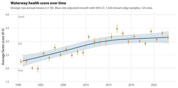
The naive linear trend is 0.43 points per decade (95% CI 0.37 to 0.48); the site-adjusted trend is 0.40 (0.30 to 0.51).
Two corrections separate those two numbers and they point opposite ways, so it is worth taking them one at a time. Allowing for site composition alone takes the trend to 0.36: ignoring it overstates the improvement by about 17%, and that is the direct measure of how much of the apparent trend is the monitoring network changing shape. Allowing for year-to-year variation as well puts about 11% of it back, at 0.40, which is the figure the rest of the chapter uses. The difference between the naive trend and the final one is the residue of those two movements rather than a measure of either, and it is why the rest of the chapter uses mixed models rather than annual averages.
The fitted trajectory rises from about 2.28 at the start of the record to about 3.15 at the end: 0.88 score points, 88% of a rating class, from the lower part of Fair into Good. But the rise is not steady.
5.5.2 Where does the improvement stop?
The split point is not a presentational detail. It decides whether the improvement is something that had already finished before the current program began, or something that overlaps with it. So it is estimated rather than assumed, with the segmented package (Muggeo 2003), on a model carrying a fixed effect for every site.
It lands at 2014.4, and that is the sturdiest number in the chapter. It is the same answer from every starting value tried (2004, 2007, 2010 and 2013); drop any single year of the record and it moves only between 2014.0 and 2014.5; and it is unchanged by adding the climate covariates, by adding SIGNAL-SF coverage, by throwing out the two chironomid years, by keeping only sites with ten or more samples, and by putting the riffle samples back in. It is not the effort curve seen through the rating, either — fit the same hinge to the number of animals per sample and that series breaks at 2018.4, 4 years later.
Where it lands is solid. How precisely it is located is not, and the two are easy to conflate. Profiling the likelihood of the two-line model over a grid of candidate breakpoints, with the site and year random effects that every other number here carries, puts the change at 2014.5 with a 95% interval of 2010.5 to 2017.25 — close to seven years wide. segmented itself reports a much tighter 2012.4 to 2016.4 (standard error 1.02 years), but it has to be fitted with a fixed effect for every site and no year effect at all, which prices the 30–90 samples of a field round as independent observations of that year. That is the mistake Section 5.4.2 is about, and it narrows intervals here as it does everywhere else. The wider one is the interval to use.
So the changepoint this report quotes is a hybrid, and it is worth saying so once. The estimate is segmented’s, because that is the fit every robustness check in the paragraph above was run against; the interval is the profile’s, for the reason just given. The two estimates are 0.1 of a year apart — 2014.4 and 2014.5 — and fall in the same calendar year. What is actually split at is that year, 2014: the before-and-after eras in this chapter, and the change-of-slope term chapter 7 tests on the water quality series, both use the whole year, so neither moves whichever of the two decimals is quoted. Nothing in this book is split at a tenth of a year.
A slope change is still real, and 2010 still sits outside the interval for where it happened — by six months rather than by nearly two and a half years.
Is this the same event as the turn in effort-standardised richness? The honest answer is that it depends on the estimator, and that the two are different behaviours whichever date is used.
Chapter 3’s fitted smooth (Section 3.4, Figure 3.2) stops rising at 2012.1 and falls from there, and 2012.1 sits inside the 2010.5–2017.25 interval above — so on that reading the two dates are not separable, and no test on this record will separate dates that close. But the smooth is a hump with two peaks, and forcing a single break through the whole rarefied series instead lands the turn in the early 2000s, two decades earlier: a one-break model calls the end of the early rise the turn, while the smooth calls the start of the recent fall the turn. Both features are in the same curve, and neither is the composite’s changepoint by construction. Quote the date with the model that produced it.
They are certainly not the same behaviour. After the changepoint the health score plateaus — -0.12 points per decade, an interval that contains zero — while standardised richness over 2010–2024 falls, -0.85 families per decade (-1.65 to -0.05), on an interval that does not. A flat score over a falling richness component is a composition change, not a stalled recovery, and Section 5.7 is where the components are separated. Read the two together: what stopped in about 2014 was the improvement; what continued was a decline in one of the four things the score is made of, offset by a sensitivity component that did not fall with it.
How strongly supported is the hinge? Well, but not overwhelmingly. Against a single-slope model, with the site and year random effects that every quoted number in this chapter carries, a change of slope at 2014 is worth a likelihood-ratio chi-square of 9.67 on 1 degree of freedom.
Reading that straight off a chi-square table gives p = 0.002, and that figure is too flattering, for a reason worth spelling out because it is easy to miss. The year the slope changes was not nominated in advance — it was found in these same rows, by trying every candidate year and keeping the best one. A test that gets to pick its own best answer and is then scored as though it had only ever looked at one place will look more impressive than it is. So the test was redone the honest way: simulate 10,000 records from the no-change model, and for each one take the largest chi-square over all 29 candidate breakpoints from 2005 to 2019. Under no change at all, that largest chi-square exceeds 3.8 — the textbook 5% cut — about one time in 6, and its 95th percentile is 6.5. The observed value to set against that is not the 9.67 above — that is the chi-square at the round 2014 — but the largest over the same grid the simulations search: 10.1, attained at 2014.5. A test that gets to pick its own best answer has to be scored against a null that gets to pick too, and both sides of the comparison now do. 104 of the 10,000 simulated no-change records beat it — 1.0%, with a 95% interval of 0.9% to 1.3%, because a counted proportion carries an uncertainty like anything else counted. So the hinge is worth about p = 0.01, not p = 0.002: an order of magnitude weaker than the table reading, and still a real slope change. There is no third digit, and that is a property of the method rather than a hedge — buying one would take a hundred times as many simulations, and nothing here would move if it did.
Smaller p-values again come from tests that leave the year effect out, and those price a whole field round as though its samples were independent (Section 5.4.2).
| Period | Samples | Sites | Change per decade | 95% CI |
|---|---|---|---|---|
| Whole record, 1998-2024 | 1,503 | 125 | 0.40 | 0.30 to 0.51 |
| Before the changepoint, 1998-2013 | 776 | 101 | 0.58 | 0.40 to 0.76 |
| After the changepoint, 2014-2024 | 727 | 77 | -0.12 | -0.46 to 0.22 |
| 2010-2024 (administrative split, retained for continuity) | 943 | 84 | 0.06 | -0.13 to 0.25 |
So: the creeks improved strongly from the late 1990s until about 2014, and nothing has been detectable since. Splitting at the estimated changepoint rather than at 2010 (Table 5.3) makes the early rise half again as steep — 0.58 points per decade against 0.38 when the record is cut at 2010 — because 2010 sits inside the steep part of the rise and drags its tail into the “later” period. It also moves roughly four years of the improvement out of the “already finished” column and into the window your current program has been running in, which is the difference that matters for reading it.
The second half of that needs stating carefully, and it is the half most likely to be misquoted. The interval for the recent period includes zero, but it is wide, and it is not symmetric about zero — so a bound on it has to be given a direction. The data since 2014 are still consistent with a decline as large as 0.46 points per decade, or with an improvement as large as 0.22. Over the longer and better-powered 2010–2024 window the corresponding bounds are 0.13 and 0.25. This is an absence of detectable change, not a demonstration of stability. A real improvement of a fifth of a score point per decade since 2010 would have gone unnoticed by a network of this size. If you want to be able to say “nothing has changed” and mean it, that is a monitoring-design question rather than an analysis one, and chapter 16 is where it is taken up.
There is a test of the plateau that this chapter cannot run on its own. If a water quality parameter showed the same shape — a rise to about 2014.4 and then nothing — the two could be tested against each other. Chapter 6 has nothing to test against: ten of its eleven parameters have no established trend in level to bend. The series that does move is the rate at which measurements fall outside the desirable ranges, and chapter 7 splits that one at this chapter’s changepoint (Section 7.4).
5.5.3 Does the trend survive the climate?
The record starts inside the Millennium Drought and ends after the wettest years in the series (chapter 4). Wet years alone could manufacture an apparent improvement.
| Term | Estimate | 95% CI |
|---|---|---|
| Time (per decade) | 0.39 | 0.28 to 0.49 |
| SPI-12 (per 1 unit wetter) | 0.04 | -0.02 to 0.09 |
| Recent rain (per e-fold increase in 30-day rainfall) | -0.04 | -0.08 to -0.01 |
It does — and the usual way of showing that is the weakest way available, so two stronger arguments are given instead.
Adding the 12-month standardised precipitation index and recent rainfall moves the trend only from 0.403 to 0.387 points per decade. On its own that proves very little: “I added the covariate and the coefficient barely moved” is exactly what you would see if the covariate were badly measured, collinear with time, or simply the wrong covariate. Two of those three do not apply here — SPI-12 is only weakly correlated with time (r = 0.22) and it is the standard index for this question. The measurement objection is the one with force, because attenuation in a badly measured covariate pushes the answer towards “not the climate” for free. It is also small by construction: 48 of the 1,503 samples — 3% — carry a regional-mean climate series rather than their own grid cell, and every one of those is at a site with no delineated catchment.
First, and decisively, climate cannot arithmetically account for the change. Fit SPI-12 with no time term at all, so that it absorbs every scrap of the improvement it possibly can: the coefficient is 0.054 points per unit of SPI-12, with an upper 95% bound of 0.116. Mean SPI-12 rose by 0.41 units between 1998–2006 and 2007–2024, while the mean score rose by 0.70 points. At the upper bound of an unconstrained climate coefficient, the wetting can account for 0.047 points — at most 7% of the observed change. To explain all of it, SPI-12 would need a coefficient of 1.71 points per unit — about 15 times its own upper bound.
Second, comparing like with like says the same thing. Restricting to the 10 years whose mean SPI-12 is below −0.3 — comparably dry years spread right across the record (2002, 2003, 2004, 2006, 2007, 2009, 2014, 2016, 2018, 2019) — the improvement is 0.46 points per decade (0.24 to 0.69, 512 samples across 10 years), which is if anything larger than the full-record trend and larger than the 0.39 of the remaining years. Do not read anything into the gap between the two: fitted directly as an interaction it is 0.01 points per decade (-0.23 to 0.26), which is nothing. The point is that the dry-year trend is not smaller, which is what the drought explanation predicts. Health did not fall back during the 2017–19 drought either: 2018 had a mean SPI-12 of -1.68 and a mean score of 3.18, against 3.00 in the wet 2017.
Taken together: the improvement is not the drought breaking. Dry years late in the record score much better than dry years early in it, and no plausible climate coefficient can close the gap. That is a statement about the average factor score, though, and the score is a blunt instrument — Section 5.6 shows that a substantial part of the rise has a non-ecological explanation, and Section 5.7 shows the components behaving quite differently from one another.
One incidental result in the climate table deserves a line of its own, because it is a methodological finding rather than an ecological one. The 30-day rainfall coefficient is negative (-0.04 points per e-fold increase, 95% CI -0.08 to -0.01): samples taken shortly after rain score measurably lower. Small, but plausibly an artefact of the catch rather than of the creek — a scouring effect on what the net picks up rather than a change in the community.
You do record flow condition on the field sheet, and have since 2008: the free-text water_level box on the site description sheet holds an ordered flow-state scale, and chapter 9 (Section 9.3.3) sets out how it was normalised into one. So the model can be run — both for whether flow state moves the score in its own right, and for the obvious question underneath the rainfall result: is the post-rain deficit just “the creek was running high on the day?”
Flow state does move the score — but not along the scale, so how you enter it decides what you find. On the 921 samples that carry one, treat the six levels as a number, as though each step were the same size of the same thing, and you get a null: -0.001 points per step (95% CI -0.04 to 0.04, p = 0.94). Let the six levels take their own values instead and they are worth a chi-square of 14.55 on 5 degrees of freedom, p = 0.012.
What carries that is one step, at the bottom. Samples taken when the creek was not flowing score -0.28 points lower than samples taken when it was (95% CI -0.48 to -0.09, p = 0.004) — about 0.32 of a standard deviation of the score, on 39 no-flow samples at 19 sites. The five flowing levels are not distinguishable from one another at all. A straight line drawn through six levels averages that step away to nothing, which is the whole of why the first fit reads as a null. None of this touches the headline: the trend on these samples is 0.19 points per decade with no flow term and 0.17 with the six levels free, and the flow record only begins in 2008, after most of the rise.
The rainfall question is a separate one, and there the null holds. Put flow state alongside the climate terms and the 30-day rainfall coefficient does not move (-0.079 to -0.085 points per e-fold) — both of those are on the 921 flow-recorded samples, which is why they are larger than the -0.04 in Table 5.4; the comparison that matters is between the two, not with the full set. So whatever the post-rain deficit is, it is not simply “the creek was running high on the day”.
Worth knowing that the no-flow step is not a curiosity of this chapter. Chapter 6 finds flow state the strongest visit-level predictor of dissolved oxygen in the record (Section 6.7), chapter 9 finds it moves community composition (Section 9.6.1), and chapter 13 finds the same step in the published rating (Section 13.5.6). Three chapters, one channel: a creek that was not running on the day it was sampled reads worse on nearly everything we measure, and that is a condition-on-the-day effect rather than a statement about the creek.
One last thing that could have manufactured a trend and did not. Sampling is not spread evenly through the year — 83% of samples are taken between January and June — and the sampling calendar has drifted over the record, which is the largest single confound in the water quality series (Section 3.7.1). It is not one here: no seasonal contrast in the health score is distinguishable from zero, and adding season moves the trend from 0.40 to 0.39 points per decade. The GAM keeps a cyclic smooth of day of year anyway.
5.5.4 The rating categories
The average factor score is the analyst’s variable; the rating is what appears in the Waterways Health Snapshot. Figure 5.2 is the same story in the units you publish.
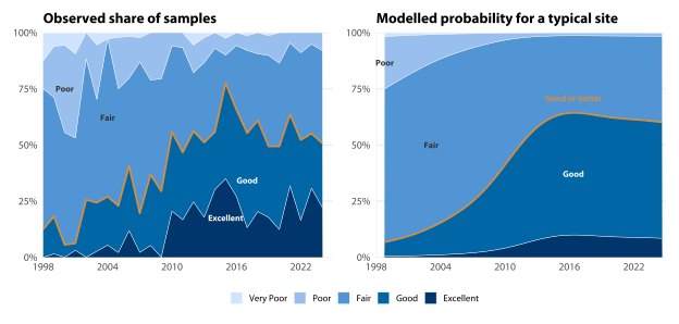
In the first five years of the record, 32% of stream edge samples rated Poor or Very Poor and 13% rated Good or Excellent. In the last five years those figures are 8% and 54%. The share of samples in the two worst rating classes has fallen by about three quarters, and the share rated Good or Excellent has quadrupled. The caveat on the left panel matters, though: part of that shift is the network expanding into different creeks, which is exactly why the right-hand panel is drawn. And the same caveat as everywhere else applies — some of the movement in the two count-based factors is the laboratory, not the creek (Section 5.6).
5.5.5 Robustness: does the answer depend on the choices?
Every alternative specification we could think to try, refitted.
| Specification | Samples | Sites | Per decade | 95% CI |
|---|---|---|---|---|
| Primary: streams, edge, site and year random effects | 1,503 | 125 | 0.40 | 0.30 to 0.51 |
| Site random effect only (no year effect) | 1,503 | 125 | 0.36 | 0.32 to 0.41 |
| Random slope in time by site | 1,503 | 125 | 0.41 | 0.30 to 0.52 |
| Adding climate covariates (SPI-12, 30-day rain) | 1,503 | 125 | 0.39 | 0.28 to 0.49 |
| Adding SIGNAL-SF coverage | 1,503 | 125 | 0.42 | 0.30 to 0.53 |
| Adding recent catchment fire | 1,455 | 117 | 0.41 | 0.30 to 0.52 |
| Fire extent, on the seasons FESM covers (2013-) | 730 | 77 | -0.07 | -0.42 to 0.28 |
| Fire severity instead, same FESM-window rows | 730 | 77 | -0.05 | -0.38 to 0.29 |
| Adding log sample abundance | 1,503 | 125 | 0.28 | 0.18 to 0.37 |
| Edge and riffle samples together | 1,826 | 125 | 0.34 | 0.24 to 0.44 |
| Core reporting sites only | 583 | 27 | 0.37 | 0.26 to 0.47 |
| Excluding all relocated site pairs | 1,178 | 98 | 0.40 | 0.30 to 0.51 |
| Excluding fire-affected catchments from 2020 | 1,467 | 125 | 0.41 | 0.31 to 0.51 |
| Excluding the chironomid-affected years 2000-01 and 2008-09 | 1,327 | 123 | 0.36 | 0.26 to 0.47 |
| Balanced panel: sampled every year 2012-2024 | 237 | 14 | 0.10 | -0.31 to 0.51 |
| Sites with at least 10 samples | 1,198 | 62 | 0.40 | 0.29 to 0.50 |
| Before the changepoint, 1998-2013 | 776 | 101 | 0.58 | 0.40 to 0.76 |
| After the changepoint, 2014-2024 | 727 | 77 | -0.12 | -0.46 to 0.22 |
| 2010-2024 only | 943 | 84 | 0.06 | -0.13 to 0.25 |
| Wetlands only (separate band table) | 208 | 9 | -0.03 | -0.28 to 0.21 |
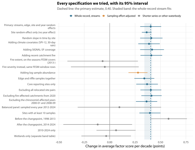
Six things stand out, and Figure 5.3 — the same twenty rows drawn as estimates with their intervals — carries four of them at a glance.
- Almost nothing changes the whole-record answer. Climate covariates, SIGNAL-SF coverage, recent fire, riffle samples, restricting to core reporting sites, dropping the relocated pairs, dropping the burnt catchments after 2019 and dropping the four years in which chironomid recording is known to be irregular all leave the estimate between 0.34 and 0.42 points per decade. The improvement over the record as a whole is not fragile.
- One specification does change it: sampling effort. Adding log sample abundance drops the estimate to 0.28 points per decade (0.18 to 0.37), a reduction of about 31%. That row is not a robustness check like the others — it is the finding, and Section 5.6 is about it.
- What the year random effect costs is precision, not the answer. Site alone gives 0.36 points per decade (0.32 to 0.41); site and year give 0.40 (0.30 to 0.51), on an interval more than twice as wide. The second is the honest one and it still excludes zero by a wide margin.
- The balanced panel agrees with the recent-period result because it cannot disagree with anything. The 14 stream sites sampled in every year from 2012 to 2024 give 0.10 points per decade (-0.31 to 0.51) on 237 samples — an interval spanning half a score point per decade in each direction. It is the only balanced design the network makes available, and it is not a strong one.
- The wetlands are not doing what the streams are doing. The wetland row is -0.03 points per decade (-0.28 to 0.21) on 208 samples at 9 sites — a flat null, not a small improvement. That is chapter 11’s finding and chapter 11’s to interpret (Section 11.6); the row is here so Table 5.5 does not silently omit the other waterbody type, and the two are the same specification on the same samples.
- The riffle row is a direction, not an estimate. The 1,826 samples in “edge and riffle together” include the riffle samples, which are scored against bands built from edge samples only and sit about a quarter of a point above the edge sample taken beside them (Section 3.6.1). Almost all of them are pre-2008, so they depress the early years and make the improvement look larger. The row is in Table 5.5 because leaving it out would hide which way that pushes, not because those scores are inside the band table’s domain.
Three of the rows need a note. The two FESM rows are deliberately paired, because the severity covariate only begins at the 2013–14 season, so they are a shorter series as well as a different model — and the extent row on the same rows is what makes the severity row readable. On those 730 samples the trend is -0.07 points per decade with fire as extent and -0.05 with fire as severity: the same answer. The 2010–2024 row is not the same answer in the sense of the same estimate — it is 0.06, on the other side of zero — but all three intervals contain zero, so none of the three is distinguishable from no trend at all, and that rather than the point estimates is what the three have in common. What moves the estimate is the window, not the covariate. That is not a statement that the two fire measures are equivalent — Section 4.4.4.1 compares them against the rating directly and severity wins by a clear margin. Both are true, because a covariate can matter a great deal for the level of a site’s score while adding nothing to a trend estimated across sites that mostly did not burn.
And “adding SIGNAL-SF coverage” is a weaker control than it looks. prop_count_no_sf_grade is the share of a sample’s individuals carrying no SIGNAL-SF grade, and chironomids are the largest single ungraded group. In 2000–01 and 2008–09 — when chironomids were recorded coarsely or not at all — that column is measuring identification practice rather than grade coverage (Section 3.5). Adding it is still worth doing, and it moves the trend from 0.40 to 0.42, but in four of the 26 years it is partly controlling for the wrong thing. The “excluding the chironomid-affected years” row is the check that does not have that problem.
5.6 About a third of the improvement is inseparable from the animal count
This is the most important qualification anywhere in this work, and it has to travel with the headline rather than behind it.
Chapter 3 diagnoses the cause and this section is what it does to the answer. The short version of the diagnosis (Section 3.4): the number of animals recorded per sample has roughly doubled over the record, with the rise concentrated in 2008–2011 — the same window in which the health score rose fastest. Two of the four scoring factors are counts of families, and the more animals you look at, the more families you find. Neither database records a subsampling protocol or a target pick count, so nobody can currently say whether the creeks hold more animals or the laboratory is picking more of each sample.
| Period | Measure | Samples | Change per decade | 95% CI | Verdict |
|---|---|---|---|---|---|
| 1998–2024 | Families recorded | 1,179 | 1.91 | 0.95 to 2.87 | rises |
| 1998–2024 | Families per 50 individuals | 1,179 | 0.05 | -0.39 to 0.50 | no net change |
| 1998–2024 | EPT families recorded | 1,179 | 0.96 | 0.67 to 1.24 | rises |
| 1998–2024 | EPT families per 50 individuals | 1,179 | 0.58 | 0.36 to 0.79 | rises |
| 2010–2024 | Families recorded | 790 | -1.49 | -2.76 to -0.22 | falls |
| 2010–2024 | Families per 50 individuals | 790 | -0.85 | -1.65 to -0.05 | falls |
| 2010–2024 | EPT families recorded | 790 | 0.07 | -0.57 to 0.71 | no net change |
| 2010–2024 | EPT families per 50 individuals | 790 | 0.13 | -0.41 to 0.66 | no net change |
The number of families recorded has risen; effort-standardised richness has not — and the flat whole-record figure is the average of a rise and a fall, not the absence of both. Raw family counts rise 1.91 families per decade (0.95 to 2.87). Standardised to a fixed count of 50 individuals and a strict family list, the whole-record trend is 0.05 families per decade (-0.39 to 0.50) — no net change across the 26 years of macroinvertebrate sampling.
But standardised richness has been falling for a decade. Over 2010–2024 the same measure falls -0.85 families per decade (-1.65 to -0.05), an interval that excludes zero, and the raw count falls with it (-1.49, -2.76 to -0.22) — so it is a decline in the creeks and not an artefact of standardising. Both periods are in Table 5.6 above, and chapter 3 traces the same shape through the fitted smooth (Section 3.4).
The EPT result is different, and it survives. Raw EPT family counts rise 0.96 per decade; standardised to 50 individuals they still rise 0.58 (0.36 to 0.79). More of the animals in a Blue Mountains stream sample are mayflies, stoneflies and caddisflies than were in the 2000s, and that is not a counting artefact.
On the health score itself the cost is about 31%. Adding log sample abundance to the headline model drops the trend from 0.40 to 0.28 points per decade (0.18 to 0.37). So the improvement is not a mirage — two thirds of it is still there with the number of animals counted held fixed — but a third of it rides on the animal count, and the whole of the apparent gain in family richness does. Whether the count went up because the laboratory started picking more or because the creeks hold more is the one thing that would tell you what that third means, and it is the one thing the record does not say.
Three things are worth being precise about, because this result gets quoted.
- The two rarefied numbers differ from the raw ones in two ways at once. The “recorded” figure is your published
n_families; the standardised figure is rarefied richness on a strict family list. So the fall from 1.91 to 0.05 is effort and the chironomid counting convention, not effort alone. Chapter 3 separates the two (Section 3.4), and both pieces are real. - %EPT is the least effort-sensitive of the three factors that have been tested, not an immune one. About 18% of its trend goes when the number of individuals counted is controlled for, and it correlates with sample size at r = 0.30 within years (Section 3.4.4). Treat it as the most trustworthy of those three with that caveat, and do not use it as a clean effort-independent anchor. There is not one in this dataset. The fourth factor, SIGNAL-SF, is a mean grade rather than a count, and it has not been tested on this axis anywhere in this report — a deeper pick adds families and so can move a mean of family grades, but nobody here has measured whether it does. It is untested, not measured to be clean, and the ranking above is therefore over the three that were measured.
- Rarefaction discards a selected subset. The 324 samples too shallow to rarefy to 50 individuals are concentrated in the early years and score about a point lower than the ones retained. Chapter 3 runs three checks against that and all three are reassuring — the answer is the same at every depth from 20 to 100, an effort control that discards nothing agrees, and the discarded samples are improving too — but the selection is real, and the rarefied series is not a random sample of the record.
What this changes downstream. Three of the four rating factors are measurably effort-sensitive and two of them badly — the fourth is untested on this axis rather than clean — so the rating moves with how many animals end up in a sample, whatever is driving that; the bands were calibrated on 2012–2015, the most thoroughly processed part of the series. That leaves two ways out — fix the pick count in the protocol, or rarefy before scoring — and it is worth deciding which. Chapters 13 to 16 take that up, and chapter 3 explains why we rarefy to 50 for research and 20 for rating work (Section 3.4.3.3). For community analysis the exposure is much lower — shares and distances are built from proportions, and picking twice as many animals leaves a proportion unchanged in expectation (Section 3.4.6) — which is why chapters 8 and 9 are far less affected by this than this chapter is.
5.7 Question 2 — the four components
The health score averages eight numbers: four factors, each scored against an urban and a reference comparison. The averaging is what hides the result in this section, so this is the section that argues for reporting the factors beside the total.
| Component | Mean value | Change per decade | 95% CI |
|---|---|---|---|
| SIGNAL-SF | 6.91 | 0.05 | -0.01 to 0.10 |
| SIGNAL-SF, adjusted for grade coverage | 6.91 | 0.05 | -0.01 to 0.11 |
| SIGNAL 2 (complete coverage) | 4.79 | 0.22 | 0.14 to 0.30 |
| Number of families (the published count) | 15.76 | 2.45 | 1.42 to 3.54 |
| Number of families (strict count) | 12.63 | 1.80 | 1.00 to 2.65 |
| Number of EPT families | 4.19 | 1.11 | 0.80 to 1.44 |
| %EPT | 45.61 | 9.94 | 6.94 to 12.89 |
The dispersion check behind the model choices in Table 5.7. DHARMa::testDispersion gives 0.92 (p = 0.38) for the published family count and 0.94 (p = 0.55) for the strict count, so Poisson is right for both. EPT family richness is materially under-dispersed (0.66, p < 0.0001) — it is bounded above by a small number of families and behaves more like a binomial count — so it is fitted as a generalised Poisson. Under-dispersion errs the safe way, making Poisson intervals too wide rather than too narrow, but the corrected model is the one reported.
5.7.1 Do they move together? No — and that is the finding
| Component | 1998-2024 | 1998-2013 | 2014-2024 |
|---|---|---|---|
| SIGNAL-SF | 0.05 (no change) | -0.03 (no change) | 0.16 (no change) |
| SIGNAL-SF, adjusted for grade coverage | 0.05 (no change) | -0.02 (no change) | 0.14 (no change) |
| SIGNAL 2 (complete coverage) | 0.22 (up) | 0.39 (up) | 0.18 (no change) |
| Number of families (the published count) | 2.45 (up) | 4.51 (up) | -1.97 (down) |
| Number of families (strict count) | 1.80 (up) | 4.05 (up) | -1.92 (down) |
| Number of EPT families | 1.11 (up) | 1.99 (up) | 0.00 (no change) |
| %EPT | 9.94 (up) | 14.53 (up) | -1.00 (no change) |
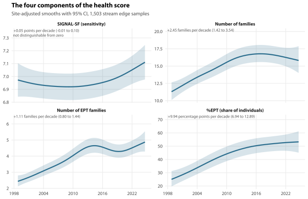
Read the whole-record column of Table 5.8 first, because that is where the evidence is. Over the full record five of the seven components rise, and the two that do not are SIGNAL-SF and SIGNAL-SF, adjusted for grade coverage. That is this section’s finding rather than an aside. The five that do rise do so for different reasons and by magnitudes that are not comparable:
- The published family count rises about 2.45 families per decade, and almost none of it survives standardising for the counting convention and the number of animals processed: on the 1,179 samples deep enough to rarefy, the same rise is 1.91 families per decade as recorded and 0.05 standardised. Standardised for both, richness shows no net rise over the record — and falls 0.85 families per decade over 2010–2024 (Section 5.6).
- %EPT rises about 9.94 percentage points per decade, and rarefied EPT richness rises with it. This one is mostly real: about 18% goes when the number of individuals counted is held fixed (Section 3.4.4), and the rest does not.
- SIGNAL 2 rises 0.22 points per decade while SIGNAL-SF rises only 0.05 (-0.01 to 0.10, not distinguishable from zero). The two sensitivity indices disagree: one of them moves and the other cannot be shown to move at all. The two slopes are not worth expressing as a ratio — the denominator is the interval just quoted, so a ratio to it has no finite bound. And the reason is structural rather than statistical: SIGNAL-SF has no grade for the tolerant taxa that dominate a degraded sample, so it barely responds to the tolerant-to-sensitive shift that has actually happened. Chapter 8 (Section 8.6.1) sets out the mechanism.
So the composite is a poor instrument. The four factors do not point in opposite directions; the problem is that one of them is largely a measure of laboratory effort, one is a real compositional signal, and one barely responds at all — and averaging gives each equal weight regardless. Two things follow, and both land three chapters away: the eight published scores carry about three independent dimensions rather than eight (chapter 13, Section 13.5.2), and any revised rating has to decide which factors it keeps and whether SIGNAL 2 replaces SIGNAL-SF (chapter 15). Whatever the rating ends up being, reporting the factors beside the total costs nothing and is where the information is.
The recent period tells a second, weaker story. Since the changepoint the family count has fallen — 1.97 families per decade on the published count and 1.92 on the strict count, both clearly below zero — while SIGNAL-SF has drifted upward (0.16 points per decade, 95% CI -0.01 to 0.33). Over the longer 2010–2024 window that SIGNAL-SF rise does clear zero (0.15, 0.05 to 0.24), and the family decline holds there too on the strict count (1.35 families per decade, q = 0.022). It does not hold on the published count, and the difference is multiplicity rather than biology: the published count’s unadjusted interval excludes zero by 0.00027 on the log scale and its Benjamini-Hochberg q across the seven components of that window is 0.09. It is the only claim in this chapter whose verdict turns on not correcting for multiplicity, and Section 5.6 already gives the independent reason to prefer the strict count here — the published one carries the chironomid relabelling.
Two more recent movements look like findings and are not established. %EPT and SIGNAL 2 have drifted upward since 2010 as well, and neither drift can be distinguished from ordinary year-to-year variation over so short a window: over 2010–2024, %EPT is 3.56 percentage points per decade (-1.36 to 8.37) and SIGNAL 2 is 0.13 points per decade (-0.05 to 0.31). With only a site random effect both of those intervals excluded zero; with year-to-year variation allowed for, neither does. That is not a change of sign, it is a loss of resolution — the recent window is short and the network is noisy.
The honest summary. Fewer families but more sensitive ones is a real pattern over the whole record, where the family-count rise turns out to be almost entirely artefactual and the EPT signals turn out not to be. Over the recent period the family decline holds on the strict count, is knife-edge on the published one, and the SIGNAL-SF rise is at the edge of detectability, but %EPT and SIGNAL 2 cannot be shown to have moved at all. Read the component divergence as a statement about the record, not about the last decade.
That is a community becoming more selective rather than richer — the tolerant generalists that pad out a family list are a smaller part of the assemblage. Whether that is good news depends on which taxa are going, and it is exactly the question chapter 8 is built to answer: a decline in richness driven by the loss of tolerant taxa is a recovery signal, a decline driven by the loss of everything is not. That is the single most useful test the community chapters can run on this result, and chapter 8 runs it on the effort-standardised series rather than the raw one (Section 8.6.1).
5.7.2 The chironomid sensitivity check
Chapter 3 records that chironomid identification resolution is not constant (Section 3.5): 2000 and 2001 record chironomids only to family, 2008 records none at all in any of its samples, and 2009 records them in five of thirty-six. Chironomids are a substantial share of the individuals in a normal year and one to three rows of the published family count, so dropping them inflates %EPT and lumping them deflates n_families. Any family-count or %EPT series crossing those windows has to show it is not an artefact of them, and this is that check.
| Series | With chironomids | Chironomid-free |
|---|---|---|
| Distinct taxa recorded, whole record (log per decade) | 0.150 (0.094 to 0.206) | 0.130 (0.074 to 0.185) |
| Distinct taxa recorded, 2014-2024 | -0.103 (-0.201 to -0.006) | -0.139 (-0.245 to -0.034) |
| %EPT, whole record (logit per decade) | 0.465 (0.324 to 0.607) | 0.493 (0.348 to 0.638) |
| %EPT, 2014-2024 | -0.046 (-0.422 to 0.331) | 0.007 (-0.454 to 0.468) |
Removing every chironomid from every sample before recomputing the metrics (Table 5.9) moves no direction and no verdict. The more aggressive check — dropping 2000, 2001, 2008 and 2009 from the analysis altogether — costs 10% of the headline trend (0.36 points per decade against 0.40, in Section 5.5.5) and again changes nothing qualitative. The recording artefact is real, it is worth about a tenth of the improvement, and it carries none of this chapter’s conclusions.
5.8 Question 3 — kinds of creek, and catchment imperviousness
5.8.1 Do trends differ between categories of site?
| Grouping | Category | Samples | Sites | Mean score | Per decade | 95% CI |
|---|---|---|---|---|---|---|
| Disturbance tier | Reference | 212 | 16 | 3.14 | 0.38 | 0.17 to 0.59 |
| Disturbance tier | Slightly disturbed | 325 | 21 | 3.68 | 0.55 | 0.38 to 0.72 |
| Disturbance tier | Urban | 966 | 88 | 2.53 | 0.31 | 0.22 to 0.40 |
| Classification | Reference | 212 | 16 | 3.14 | 0.38 | 0.17 to 0.59 |
| Classification | Urban | 1,291 | 109 | 2.82 | 0.41 | 0.31 to 0.51 |
| Altitude zone | Higher altitude | 872 | 60 | 2.98 | 0.37 | 0.26 to 0.49 |
| Altitude zone | Lower altitude | 477 | 33 | 2.82 | 0.46 | 0.33 to 0.59 |
| Major catchment | Burragorang | 417 | 26 | 2.92 | 0.42 | 0.29 to 0.55 |
| Major catchment | Grose | 528 | 48 | 2.98 | 0.36 | 0.23 to 0.50 |
| Major catchment | Nepean | 521 | 48 | 2.63 | 0.40 | 0.29 to 0.51 |
Every one of the 14 category rows in this family — the ten in Table 5.10 above plus the four imperviousness bands below — excludes zero, and all 14 still do after Benjamini–Hochberg adjustment across the family (largest adjusted p-value 3.7^{-4}). One of them, however, is not a distinct test: Classification / Reference is the same fit on the same samples as its counterpart under another grouping, because classification is tier with the two disturbed levels merged. So the family holds thirteen distinct trends, and the adjustment is run over those thirteen rather than over all fourteen rows; the duplicated row carries its counterpart’s adjusted p-value, which is the same test’s. Nothing turned on the distinction either way: the largest adjusted p-value is 3.7^{-4}, so no adjusted decision is anywhere near a boundary and the size of the family could not have moved one. There is no borderline mass here for selective reporting to have created.
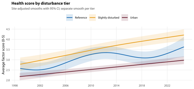
- All three tiers improved. Reference sites 0.38 points per decade (0.17 to 0.59, 16 sites), slightly disturbed 0.55 (21 sites), urban 0.31 (88 sites).
- Urban sites are not catching up. The urban trend is indistinguishable from the reference trend (interaction 0.01, 95% CI -0.14 to 0.16). Across the record as a whole the average reference site scores 0.46 points above the average urban site — a single number with no time dimension in it, and a mean over sites rather than over samples, because the tiers are unbalanced in how often each creek was visited. The gap that does have one is the distance between the fitted curves in Figure 5.5, and it runs 0.40 points at the start of the record to 0.65 at the end: if anything wider, not narrower, and the 0.10 points per decade that implies is inside the interval on that interaction, so the widening is not something this record can tell apart from no change.
- The ‘slightly disturbed’ sites improved fastest, by 0.26 points per decade more than reference sites — and they also score highest, 3.77 on average against 2.95 at the reference sites, at every year of the record (Figure 5.5). The tier names do not rank the creeks; worth knowing before anyone reads the reference tier as the best the network has. These are the urban-catchment sites that fall on the good side of your own 5% band edge — which was drawn on the connected fraction, not on the total imperviousness used here, so do not read the 5% as a number on this chapter’s x-axis. They are where recovery is most plausible on physical grounds: enough urban influence to have degraded, little enough to recover. It is also the imperviousness result seen from the other side. These sites have a median of 5.3% catchment sealing against 0.0% at the reference sites — medians over the 21 of 21 slightly disturbed and 14 of 16 reference sites that have a delineated catchment, since a catchment statistic can only be taken over sites that have one. Across that stretch of the gradient health does not fall — see Health against catchment imperviousness below, where the same fact turns up as a low end the data cannot resolve.
- Altitude and catchment make little difference. Lower-altitude sites improved slightly faster than higher-altitude ones, and the three major catchments are within 0.06 points per decade of each other. Neither is a management signal.
A caution on the reference tier, and it is not a small one. 9 of the 15 delineated reference catchments burnt over 90% of their area in the 2019–20 fires (Section 4.4.3.1), and several had already burnt in 2013–14. So the reference trajectory after 2020 is a post-fire trajectory, and the wide ribbon around it in Figure 5.5 reflects sampling uncertainty only — not the fact that the benchmark itself moved. That matters well beyond this chapter: reference condition is what the published bands are calibrated against, and two of the four calibration years (2012–2015) precede the fires. Any re-derivation of the bands has to decide explicitly whether reference condition means pre-fire or post-fire, and chapter 14 is where that decision lands.
5.8.2 Health against catchment imperviousness
| Group | Samples | Sites | Median sampling year | Mean health score | Currently monitored |
|---|---|---|---|---|---|
| Sites with a delineated catchment | 1,455 | 117 | 2013 | 2.87 | 80% |
| Sites without one | 48 | 8 | 2001 | 2.46 | 0% |
This section is not run on a random subset of the network. The 8 stream sites with no delineated catchment — 27GLNR, L13, L4, M23, P7, U13, U39, U44 — are the legacy network (Table 5.11). Their median sampling year is 2001 against 2013 for the rest, and 0% of their samples come from currently monitored sites. So everything here is effectively a statement about the modern network. That is not a reason to distrust the dose-response relationship, which is cross-sectional, but it is a reason to be careful with the trend comparisons that follow.
Being precise about why those eight have no catchment: it is not that they have no coordinates. Every one of the 137 register sites holds an easting and a northing. These eight are withheld from delineation because their recorded position cannot be resolved onto the stream network well enough to trust the catchment that would come out of it.
| Catchment imperviousness | Predicted health score | Rating | Without a site effect | Naive minus site effect | Sites at or above |
|---|---|---|---|---|---|
| 0% | 3.26 | Good | 3.40 | +0.13 | 117 |
| 2% | 3.19 | Good | 3.34 | +0.14 | 97 |
| 5% | 3.09 | Good | 3.24 | +0.16 | 86 |
| 10% | 2.91 | Fair | 3.06 | +0.15 | 63 |
| 20% | 2.56 | Fair | 2.48 | -0.08 | 27 |
| 30% | 2.20 | Fair | 2.19 | -0.02 | 8 |
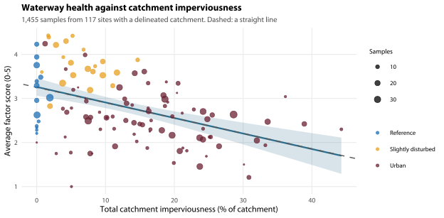
Before reading anything off that curve, one methodological point. Imperviousness is a property of a site, not of a sample, and these 1,455 samples come from only 117 sites — a median of 10 samples each. A smooth fitted without a site random effect treats each sample as an independent observation of its site’s catchment, which makes the confidence ribbon about 1.92 times too narrow. Worse, the most impervious sites are the ones with the most samples, so the two fits part company at the ends of the gradient rather than in the middle. Across the last 10 percentage points the sample-level fit loses 0.029 health-score points per percentage point against the site-effect fit’s 0.035 — the flatter of the two exactly where the support is thinnest — while across the whole gradient it falls 1.21 points against 1.06, which makes it the steeper of the two overall. What the missing site effect does is misplace the shape, not flatten it. The fifth column of Table 5.12 is the size of that disagreement at each level, and it is the size of the problem.
The two fits that do respect the site structure agree with each other to within 0.01 points everywhere: the GAM with a site random effect, and an independent smooth of the 117 site means, weighted by the precision of each mean rather than by the number of samples behind it — 1/(τ² + σ²/n_i), with the variance components read off the mixed model, because sample count is the correct weight only when creeks do not differ from the fitted line at all, and here they differ more than the samples within them do. Both keep falling across the whole range.
| Range of catchment imperviousness | Health score lost across the range | Per percentage point |
|---|---|---|
| 0% to 2% | 0.07 | 0.035 |
| 2% to 5% | 0.11 | 0.035 |
| 5% to 10% | 0.18 | 0.035 |
| 10% to 20% | 0.35 | 0.035 |
| 20% to 30% | 0.35 | 0.035 |
So the description that fits the network as a whole is a decline of about 0.035 health-score points per percentage point of catchment imperviousness (95% CI 0.024 to 0.045, on 1,455 samples from 117 sites) — from 3.26 at an unsealed catchment to 2.20 at 30% sealed, a fall of 1.06 score points, most of a whole rating class. That rate is avg_factor_score ~ imp + (1 | site) + (1 | yearf), fitted on the samples. The fall beside it is a different fit — it is read off the smooth, avg_factor_score ~ s(imp) + s(site), which carries no year term — so the two do not multiply into each other: 30 percentage points at the straight-line rate is 1.04 score points against the 1.06 the curve loses over the same span, a gap of 0.02. That gap is not curvature — the smooth is using 1.0 effective degrees of freedom, which is a straight line — but the two fits do not carry the same random effects, and the year term is the one the smooth is missing. Quote the rate or quote the total; do not quote the rate and then multiply it out. Table 5.13 sets that fitted loss beside each part of the gradient. Across the whole of that gradient the curve loses health score at one rate, not just across the middle of it: every range, from the 0% to 2% band at the unsealed end to the 20% to 30% band at the sealed one, comes out at the same 0.035 points per percentage point. No band slows down, and that includes the most sealed one — the band that bears on whether the decline eventually runs out. That constancy is the finding here. It is not evidence that there is no threshold: the column is a property of the fitted smooth, and what that smooth can and cannot rule out is what the rest of this section is about.
Is there a level of sealing at which it stops? We cannot tell you. That is the honest answer, and it is not the same answer as “no”.
Fitting a changepoint model to the site means with segmented (Muggeo 2003) does put a break in, at 30.84% total imperviousness, and the two slopes either side of it are nothing like each other: -0.041 health-score points per percentage point below the break against 0.045 above it — the decline all but stopping. But that break cannot be told apart from a straight line. Davies’ test for a change in slope (Davies 1987) gives p = 0.326, the interval on the break runs 21.39% to 40.30%, and the smooth uses 1.0 effective degrees of freedom where a straight line uses one — a straight line fitted with the same site random effect comes out slightly ahead of the smooth on AIC (2814.72 against 2814.77).
The reason not to read that as “there is no threshold” is that the test is nearly blind to one. Resample the residuals of that same weighted site-mean regression under a shape with a complete floor built into it — health falling to some level of sealing and then flat above — and refit Davies’ test to each resample. It finds the floor only 15% of the time when the floor is at 10% sealing — about one resample in 7 — and never better than 20% anywhere between 5% and 20%. The one shape it does detect reliably is health improving with sealing, which is not the shape anyone is asking about. So p = 0.326 is the failure of a test that would mostly have failed anyway, and quoting it as evidence that there is no threshold is quoting the wrong thing.
The bottom of the gradient is the part these data see least well, and it is the part a planner asks about. The whole-range slope above is fitted across the whole range; restrict the same regression to the 54 sites below 10% sealing — half the network, not a corner of it — and it is -0.013 per percentage point (95% CI -0.084 to 0.057, p = 0.71). Below 5% sealing, on 31 sites, it is 0.020 (95% CI -0.151 to 0.190, p = 0.82) — pointing the other way, but on an interval about 17 times the size of the estimate. Neither of those is a finding in its own right — the low-end interval comfortably contains the whole-range slope, so a constant decline is not refuted. But it is not shown either, and the chapter’s own tier result says the same thing from the other side: the slightly disturbed sites, median 5.3% sealed, score above the reference sites at 0.0%.
What would settle it, and it is not more sites. Run the same power calculation on a hypothetically larger network and it takes roughly 6 times the present 117 catchments to reach conventional power against a complete floor at 15%. That is not a monitoring ask; it is a statement about what a cross-sectional network of this size can do, and it belongs with the design limits rather than on a wishlist. The design that would answer the question is a catchment whose imperviousness actually changed, measured before and after — which is the same thing the stormwater-works evaluation in chapter 17 asks for.
One thing is worth pausing on, because it is a lesson about the variable rather than about the creeks. Put the modelled connected imperviousness on the x-axis instead of the total and a threshold appears, at about 16.5% connected (95% CI 10.4% to 22.7%) — Davies’ test on that scale gives p = 0.048, against p = 0.326 on the total scale above. Same sites, same health scores, same fit; one axis rejects a constant gradient and the other does not. The two measures rank the catchments identically — Spearman rho is exactly 1, because the connected model is a monotone transform of the total — so no creek has changed places. What changed is the spacing: the connected figure is convex in the total (10% total is 3.2% connected, 25% is 12.5%, and the most sealed catchment in the set, at 44%, is 29.5%), so it stretches the sealed end and compresses the unsealed one, and a constant decline per point of total sealing comes out looking like a threshold response. A threshold read off a dose-response curve can be a property of the transform rather than of the streams, which is one more reason not to write one into a planning instrument.
That also puts this analysis in a slightly different place relative to the literature. Walsh, Fletcher, et al. (2005), working on Melbourne streams, reported ecological condition declining with effective imperviousness only up to a threshold in the range 1% to 14%, beyond which no further degradation was observed. These data cannot resolve an exhaustion point either way. The decline here is close to linear across a range running to 44% sealed, but the interval on the upper part of that range is wide, the sites up there are few, and the test for a change of gradient is the near-blind one described above. So this is neither a confirmation of Walsh’s result nor a refutation of it.
On where the harm starts, the literature is less forgiving than anything these data can support. Booth and Jackson (1997) put the onset of readily observable degradation at about 10% effective imperviousness, while noting that sensitive systems degrade well below it.
King et al. (2011) tested the low end directly, and found not a scattering of responses but a synchrony. Across 1,939 Maryland stream reaches the paper documents clear, synchronous threshold declines in 110 of 238 macroinvertebrate taxa, and puts the community-level threshold at 0.68%, 0.96% and 1.28% impervious cover in the three regions it covers, with the 95% upper limit below 2% everywhere. The change points strung out along the gradient at different levels are the positive-responding, tolerant taxa — the ones that increase — not the sensitive ones. So where the low end has been resolved properly, the community moves together, and it moves very early.
Those two numbers are not on the same axis, and should not be read as a range. Booth’s 10% is effective imperviousness — the sealed area actually plumbed into the drainage network — while King’s ~1% is total impervious cover, measured off a 30 m satellite raster. Total imperviousness is the measure this book uses throughout, under the decision recorded in chapter 4, so King is the like-for-like comparator and Booth is not.
Nor do the two thresholds sit near one another, and the direction is worth stating because it is easy to read them the other way round. Connected imperviousness is a subset of total imperviousness — the sealed area that is plumbed in cannot exceed the sealed area — and in these catchments that holds by measurement rather than by assertion: no connection measure exceeds total cover in a single delineated catchment here, and wherever there is any sealing at all both sit well below it. A catchment at 10% effective cover is therefore at 10% total cover at the very least, and on the ratios these catchments show, materially more. Booth’s onset sits far above King’s ~1% total on the axis this book measures, and King’s is by a wide margin the earlier of the two. That is an ordering and nothing more: no arithmetic here converts one into the other.
That does not overturn the no-breakpoint result above, and the two are not in competition. They sit on the same axis and disagree about where a threshold is, not about whether one can exist. Ours is a statement scoped to our own record, and the scope is the point: a threshold at about one per cent of the catchment sealed is below almost the whole of this gradient. Only 20 of the 117 sites here sit below 2% sealed at all, against a median site at 11.3%. If King’s number is right, nearly every creek in this network is already past the threshold — which is exactly what a smooth, near-constant decline with no locatable breakpoint would look like from up here. Read the two results together, not as a contradiction to be settled.
5.8.2.1 What you can and cannot key a planning decision to
Three things rule out any advice keyed to an absolute imperviousness number.
- No threshold can be located. Not because there is none — see above, where the test that would find one turns out to be nearly blind to it — but because nothing in these data says where a line should go.
- The top of the range rests on very few sites. 27 sites and 354 samples sit above 20% imperviousness, and only 8 sites above 30%. The site imperviousness quartiles are 5.0%, 11.3%, 19.7%, so the shape at the sealed end should carry very little weight.
- The absolute scale is not trustworthy. Imperviousness here is a composite: roof area is measured, from Council’s building polygons, but the paving that goes with it is a multiple of that roof set by the planning zone, and the road contribution is a cadastral road reserve times an assumed sealed fraction. Chapter 4 shows the estimate moving by a factor of two to three across defensible methods. Under a different method the whole x-axis stretches and any number written into a policy stretches with it.
What is robust is the ordering. A smooth of the rank of imperviousness explains as much of the between-site variation as a smooth of the value itself (21.8% of the deviance against 20.5%), so nothing about the relationship depends on the absolute scale. The Spearman correlation between a site’s imperviousness and its mean health score is -0.42.
Health falls with imperviousness across the network, and the ordering of catchments is usable for prioritising. A numerical threshold is not — this network cannot tell you whether one exists, and where the question has been resolved properly the answer is of no use to a planner anyway. So rank catchments by imperviousness and protect the least sealed. Drawing a planning line at a particular percentage is a policy choice, and for the three reasons above this analysis can neither support nor refute one — but the case against a line is stronger than that, and does not rest on our own null result. King et al. (2011) puts the community threshold below 2% sealed, which is under 97 of the 117 catchments in this network and far below any figure a planning instrument could sensibly be written around. A trigger set anywhere a planner would set one has already been passed. If a number is unavoidable, the honest statement beside it is that the decline is clear across the network as a whole and not detectable below about 10% sealing, where the same regression on the 54 sites below that line returns -0.013 per percentage point (-0.084 to 0.057, p = 0.71) — and that the first few per cent are demonstrably not free. That is the sentence to quote, and it is weaker than “health falls at much the same rate right across the range.” 54 of the 117 sites sit below 10% sealed; over that half of the network this record can neither show the decline separately nor refute it, so “the first few per cent are not free” rests on the whole-network slope and on King et al. (2011), not on a measurement of that stretch.
| Specification | Samples | Sites | Slope per log unit | 95% CI |
|---|---|---|---|---|
| Central imperviousness estimate | 1,455 | 117 | -0.26 | -0.37 to -0.15 |
| Lower bound of the estimate | 1,455 | 117 | -0.28 | -0.40 to -0.17 |
| Upper bound of the estimate | 1,455 | 117 | -0.25 | -0.35 to -0.14 |
| High-confidence imperviousness estimates only | 319 | 30 | -0.16 | -0.31 to 0.00 |
| High-confidence delineations only | 691 | 66 | -0.17 | -0.32 to -0.03 |
| 2010 onward only | 940 | 83 | -0.36 | -0.50 to -0.23 |
The relationship in Table 5.14 holds at either end of the imperviousness uncertainty band: -0.28 on the lower bound and -0.25 on the upper, against -0.26 on the central estimate, and none of those three intervals comes near zero. The gradient does not depend on which end of the band you take, so in that sense it is not an artefact of the imperviousness model.
It survives dropping the low-confidence catchments only in part, and the table should be read as saying so. On the 30 sites with high-confidence imperviousness estimates the slope is -0.16 (-0.31 to 0.00), which spans zero; on the 66 sites with high-confidence delineations it is -0.17 (-0.32 to -0.03), which excludes zero by 0.0284. So the check half-passes: only the high-confidence delineation subset keeps an interval clear of zero. That is a Wald interval, on a subset that gained one high-leverage site at the sealed end of the gradient, so the clearance is a margin to report and not one to build on.
The attenuation is the sturdier half of the reading, and it is not in question. Neither result is simply the smaller subset being less precise: both point estimates are also nearer zero than the full-set -0.26 — 59% and 66% of it — and the widening on its own does not account for what the intervals do, since the full-set slope carried at those two subsets’ precision would reach only -0.11 and -0.12 at its upper end and still exclude zero. The relationship attenuates under both filters as well as blurring; whatever else these two rows do, they do not reproduce the full-network slope, and that is the part of this check that fails.
Two things bear on how much weight the check should carry, and neither settles it. delineation_confidence grades a catchment on several things beyond how well the site snapped to the stream network, and on the current grading 69 of the 120 delineated catchments reach high. It is a real filter, but it is not a small one, and it is not purely a test of the imperviousness figure. And the high-confidence imperviousness subset is 30 of 117 sites; it is not range-restricted — its site imperviousness still runs from 0.0% to 38.9%, against 0.0% to 44.3% across the network — but a quarter of the network is a weak test in both directions, and it neither confirms the gradient nor refutes it.
So what this table establishes is narrower than the earlier draft claimed. The gradient on the full network, and under either bound of the imperviousness estimate, is not an artefact of the imperviousness model. Whether it is independent of how well individual catchments are graded and delineated is not settled here, and nothing above rests on its being so.
5.8.3 Does the trend differ along the gradient?
This is the question underneath the question: are the degraded catchments recovering, or only the clean ones?
| Imperviousness band | Samples | Sites | Mean score | Per decade | 95% CI |
|---|---|---|---|---|---|
| Under 5% | 381 | 31 | 3.37 | 0.50 | 0.33 to 0.67 |
| 5-10% | 275 | 23 | 3.15 | 0.49 | 0.35 to 0.63 |
| 10-20% | 445 | 36 | 2.78 | 0.40 | 0.26 to 0.53 |
| Over 20% | 354 | 27 | 2.24 | 0.25 | 0.13 to 0.37 |
Every band in Table 5.15 improved. The interaction between time and imperviousness in a single model — fitted with a random slope in time by site, so the comparison is between site trends rather than between pooled samples — is -0.035 points per decade per log unit (95% CI -0.098 to 0.028). That interval includes zero, so convergence has not happened and no direction can be read off it either way — the urban catchments have not closed the gap on the reference catchments, and there is no evidence they are closing it faster or falling further behind. If the expectation is that catchment works will show up as urban sites improving faster than reference sites, that signal is not in the data yet — which is consistent with the plateau in Section 5.5, and with chapter 17’s finding that the treatment works cannot be evaluated at all without commissioning dates.
5.9 What we can and cannot say
| Question | Answer | Confidence |
|---|---|---|
| Has overall waterway health changed? | Yes over the whole record: about +0.40 points per decade, and the fitted trajectory rises 0.88 score points — 88% of a rating class — across the 26 years of the macroinvertebrate record. The improvement ends at an estimated changepoint of 2014.4, on a profiled 95% CI of 2010.5-2017.25 — the profile is a separate fit, carrying the year effect, and puts the change at 2014.5, in the same year — and nothing is detectable since. | High for the whole-record direction, which survives all 12 whole-record specifications tested. High for where the changepoint sits — it survives leave-one-year-out and every covariate tried — but only moderate for how tightly it is located, and the hinge itself is worth about p = 0.01 (95% CI 0.009 to 0.013 over 10,000 simulations) rather than the 0.002 a chi-square table gives. Moderate for the recent period: an absence of detectable change, not a demonstration of stability. An improvement of up to 0.25 points per decade since 2010 would have been missed, and a decline of up to 0.13. |
| Is the improvement real, or an artefact? | About 31% of it disappears once the number of animals processed per sample is held fixed, and the family-count component goes almost entirely: standardised to a fixed count, family richness shows no net change over the record, and falls 0.85 families per decade (0.05 to 1.65) over 2010–2024. Whether that third is laboratory practice or creeks that really do hold more animals is not decidable from these data. | High that sampling effort inflates the count-based components. Unresolved whether the abundance rise is ecological or procedural, because no protocol was ever recorded — one document would settle it. |
| Is it the drought breaking? | No. At the upper bound of an unconstrained climate coefficient the wetting can account for at most 7% of the observed change, and comparing dry years with dry years across the record gives a larger improvement than the full record does. | High, on two arguments that do not depend on the climate covariate being well measured. |
| Have the four components changed? | Yes, and not together. Over the whole record the family-count rise is almost entirely artefactual while the EPT signals are not, and the two sensitivity indices disagree: SIGNAL 2 rises 0.22 points per decade while SIGNAL-SF cannot be shown to move at all (0.05, -0.01 to 0.10). Since the changepoint the family count has fallen while SIGNAL-SF has drifted up. | High for the whole-record divergence; moderate for the recent family decline; low for the recent %EPT and SIGNAL 2 movements, neither separable from year-to-year variation. |
| Do trends differ between kinds of creek? | All three tiers improved; urban sites did not improve faster than reference sites, so the gap has not closed. | Moderate: the reference tier is only 16 stream sites, and 9 of the 15 delineated reference catchments burnt over 90% in 2019-20. |
| Does health track catchment imperviousness? | Strongly, and close to linearly across the network as a whole: about 0.035 points of health score per percentage point of catchment sealed (0.024 to 0.045). Whether there is a threshold is undecided rather than answered — a breakpoint model puts one at 30.84% with the slope falling from -0.041 to 0.045 across it, but Davies’ test cannot separate that from a straight line (p = 0.33) and would miss a complete floor most of the time. | Moderate to high for the gradient and for the ordering of catchments. Unresolved for any absolute threshold: this network has 0.09 to 0.20 power against a complete floor, so the null is uninformative. Low for the bottom of the range, where the slope on the 54 sites below 10% sealing spans zero, and low for the shape at the sealed end, where only 27 sites sit above 20% and 8 above 30%. |
| Are degraded catchments recovering faster? | No, and there is no evidence they are recovering more slowly either. | Moderate for the absence of convergence; the interaction interval includes zero once site-specific trends and year-to-year variation are allowed for. |
5.10 Limitations of this chapter
The questions only you can answer are in the list at the top of the chapter. What follows is the shorter list of things that are limits of the analysis rather than of the record, and they should be held against everything above.
Site random effects are not site fixed effects. A random effect assumes a site’s intrinsic level is unrelated to when it was monitored. Sites added after 2016 are systematically different from those retired before 2010, so that assumption is partly violated here. The balanced-panel and core-reporting-site rows in Section 5.5.5 are the checks against it and both agree with the main result — but the balanced panel is 14 sites, so “agrees” is weaker than it sounds.
The factor-score bands were calibrated in-sample. Each of the eight factor scores is a 0-to-5 lookup against thresholds set from 2012–2015 percentiles of this same dataset, so a sample from that window is partly being scored against itself. That inflates nothing in the trend estimates, but it does mean the score is not an absolute scale, and it is one reason the chapter reports the average factor score rather than only the rating class. Chapter 14 is where those bands are re-derived.
The five rating classes are not percentiles. Very Poor through Excellent are fixed cuts one score point wide on the average of the eight factor scores — 0–0.99, 1.00–1.99, and so on to 4.00–5.00 — set in the methods document and not derived from the record at all. So the in-sample caveat above is about the 0-to-5 scores, not about where the five words fall.
12 samples recorded no animals at all and so carry no health score. They are excluded throughout. They are genuine empty samples rather than missing data — a run of them at one site would itself be a finding — but no site accounts for more than 2 of them, so nothing is being lost systematically.
And the largest one, restated because it is easy to lose in a limitations list: whether the doubling in animals per sample is ecological or procedural cannot be settled from these data, because neither database records a subsampling protocol, a pick count or a laboratory method. Both readings are reported and the analysis is run both ways (Section 5.6). It is dq:pick-count-protocol on chapter 3’s list.
| Item | Value |
|---|---|
| Data layer built | 2026-08-30 12:56 |
| R version | R version 4.4.3 (2025-02-28) |
| Primary analysis set | 1,503 samples, 125 sites, 1998-2024 (26 years) |
| Shared artefacts read | rarefied-richness, ept-effort-attenuation |
| Model fits | read from the targets graph in R/_targets.R |