| Decision and choice | Why |
|---|---|
| Program — Macro samples only; RecWQ excluded | RecWQ (recreational water quality) samples exist only from 2017 (987 samples at 8 sites, five of them shared with the Macro network). Including a site set that appears halfway through the record would put a step into every series at 2017 — the same year as an instrument change. The two programs also sample different seasons: RecWQ is 62% summer and has no winter samples at all. |
| Waterbody type — streams only | Wetlands behave differently and are scored differently. Site 922 (Wentworth Falls Lake — Jetty) is a lake carrying an Urban classification, so it reads as a stream; it is RecWQ-only and is therefore already excluded by the program filter. |
| Samples with no measurements — excluded | 718 of 2,688 tblSamples rows carry no measurement row at all (434 of them RecWQ). They are absent data, not zeros. |
| Seasonal correction — two day-of-year harmonics in every model | The sampling calendar drifted by about 3 months over the record (Section 3.7.1). Without a seasonal term, that drift is indistinguishable from a trend for every temperature-sensitive parameter. |
| Site composition — site random effect in every model | The set of sites visited changes from year to year, exactly as for the macroinvertebrate data (chapter 1). Trends are estimated within sites. |
| Field round — year random effect in every model | Everything sampled in one annual round shares the weather, the crew, the calibration of the day and the reagent batch, so the samples in a round are not independent replicates. Treating them as independent makes every confidence interval 1.2 to 3.5 times too narrow (Section 6.4.2.1). |
| Skewed parameters — modelled on the natural log | Conductivity, salinity, turbidity, alkalinity, phosphate, nitrate and faecal coliforms are bounded at zero and strongly right-skewed. Effects on these are reported as percentage change per decade. |
| Censored values — substituted at a floor, not dropped | Reported zeros mean ‘below what the method can see’, not a measurement of nothing, so they are set to a floor rather than dropped or logged to minus infinity. 7 of the 11 parameters carry one. 3 of the floors are laboratory detection limits the data layer holds, and of those only faecal coliforms is confirmed from a document; the remaining 4 are substitution points chosen here, with no documentary basis (Section 3.7.5). The censoring rate is reported alongside every result. |
6 Water quality: what changed
Blue Mountains City Council Healthy Waterways — statistical analysis
6.1 What this chapter is for
You asked whether water quality has changed, and at which sites. This chapter answers a slightly different question, because the first one turns out not to be answerable yet: what would it take to answer it?
Here is the finding, and it is a finding rather than an apology. Of the eleven parameters in the record, one shows a change over time that survives everything we can throw at it — water temperature, rising by about half a degree per decade. The other ten do not, and they fail for reasons that are all the same kind of reason. The sampling calendar drifted about 3 months. The probe was replaced twice with no day of overlap at either changeover. Something moved at the laboratory bench at least twice, and nobody wrote either of them down. The water quality record mostly measures its own methods, and once that is allowed for there is very little movement left to attribute to the creeks.
Chapter 3 diagnoses each of those changes and says, per change, how big it is and whether it can be separated from the environment. This chapter does not re-derive any of it; it states the consequences, parameter by parameter, and sets out what water quality can and cannot currently be used for — including whether it belongs in a health rating (Section 6.9). The exceedance question — how often a sample sits inside its desirable range, and what a report card may honestly print — is chapter 7.
6.2 The data behind this chapter
Each question and request below is set out again in What we need from you, with what it blocks, what an answer is worth and what it would cost you to find, ranked against every other ask in the report.
6.2.1 What this chapter uses, and where it came from
Water quality is collected in a single round each year, so everything sampled in one round shares the weather, the crew, the calibration of the day and the reagent batch. Every model here treats the round as the unit rather than the sample.
Treating the samples of a round as independent observations makes every confidence interval between about 1.2 and 3.5 times too narrow, and fixing it moves three of the eleven results, which are not three of a kind. Two change their verdict: pH and dissolved oxygen in mg/L turn out never to have been established at all, rather than established and then lost to the instrument — which is the stronger statement. The third is conductivity, whose interval never excluded zero either way but widens by the largest factor of the eleven until it runs from a fall to a substantial rise, so a null that read as reassuring becomes uninformative. It also caps what the record can do at all: 27 rounds is 27 observations of anything that varies year to year — the instrument steps, the wet-year terms, any change of slope — and that is a property of the monitoring design, not of the analysis. The same arithmetic reaches past the eleven parameters: the drift in flow state over the record, which looks decisive on a site-only fit, is not established either.
Blocks: Reading any water quality null in this chapter as evidence of stability; the size, as opposed to the existence, of anything estimated year to year. Value: moderate. Costs you: minutes. Refer to it as
dq:field-round-is-the-unit.
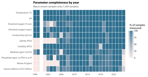
A trend is a statement about the years its own parameter was measured, and those years differ a lot: turbidity starts in 2001, phosphate in 2002, salinity in 2005, and nitrate-N and the usable coliform series in 2006.
At the other end the laboratory parameters run out early — phosphate and nitrate-N have nothing at all in the final year, alkalinity and coliforms only a dozen samples — and single years are near-empty in the middle. So “no change since 1998” is not a sentence that can be written about five of the eleven. The same unevenness sets the size of the site-level work: a site needs eight years of a parameter before it can be tested at all, which is what leaves the scan with roughly sixty sites per parameter.
Blocks: Any “since 1998” framing for turbidity, phosphate, salinity, nitrate-N or faecal coliforms. Value: low. Costs you: minutes. Refer to it as
dq:wq-parameter-coverage.
Every trend here is the macroinvertebrate program’s own water quality samples from streams, 1998 to 2025 — about 27 years of record, which is not the same 26 years the macroinvertebrate chapters run on.
The recreational program is left out: none of it predates 2017, it shares only five sites with this network, and it is 62% summer samples with no winter at all, so bringing it in would put a step into every series in the same year as a probe change. Wetlands are left out, and so are the rows that carry no measurement of any kind — those are absent data, not zeros, and nothing in either database says whether the results were never taken, never entered or lost. Every model carries a site random effect, a year random effect and two day-of-year harmonics; the seven skewed parameters are modelled on the natural log; reported zeros are substituted at a floor rather than dropped; and faecal coliforms start at 2006, because everything before the break is a different measurement (dq:coliform-break-undatable).
Blocks: Nothing — it is a statement of what the numbers count, so that anyone requoting a trend knows which record and which samples it describes. Value: low. Costs you: minutes. Refer to it as
dq:wq-trend-analysis-set.
6.2.2 What is wrong with it
The same site-level scan run conventionally — raw site-year medians, no seasonal correction, no instrument term — returns a list of significant site trends, and every large group in it is the probe or the calendar.
Most of them are “turbidity is falling at this creek” and “salinity is falling at this creek”, which are the 2017 and 2020 probe replacements. At the uncorrected 5% level the scan also flags a couple of dozen creeks where the water is apparently getting colder — that is the round sliding out of late summer and into late autumn and nothing else. Correct for season and instrument era and not one test survives. The conventional analysis is a defensible analysis, it is what the standard texts describe, and it would have sent people out to creeks where there is nothing to find. What to do about it — whether site-level water quality goes into the report card at all — is dq:site-level-reporting-decision.
Blocks: Any site-level water quality analysis run without a seasonal term and an instrument-era term. Value: high. Costs you: minutes. Refer to it as
dq:conventional-site-scan-artefacts.
Water temperature is the one parameter of eleven whose trend survives everything — about half a degree per decade — but the seasonal correction that produces it is several times the size of the trend, and your own climate grid does not confirm it.
With no seasonal term temperature is falling; with two day-of-year harmonics in, it is rising. That reversal is the sampling calendar (dq:sampling-calendar-drift), and the correction between the early and late median sampling dates is several times the whole-record trend. Eight additive specifications — six of them varying the seasonal adjustment, two varying something else entirely — agree on the direction, and so do both halves of the season-by-trend interaction that has since replaced the single rate: ten rows, and not one of them approaches zero. So the finding stands — but quote about half a degree per decade, averaged over the calendar year, and never two decimal places. The second qualification is that regional mean maximum air temperature over the same years rises much less, and is itself indistinguishable from zero. Either the creeks are warming faster than the air, or part of the estimate is left-over sampling artefact. That is worth answering, not a finding already made.
Blocks: Quoting the temperature trend to two decimal places, or as corroborated by the regional climate record. Value: high. Costs you: minutes. Refer to it as
dq:temp-trend-qualifications.
Over half the phosphate readings and over half the faecal coliform counts in the trend set sit at or below the floor we substituted, so the size of any trend in them is partly a property of that choice rather than of the water.
This is dq:zeros-are-nondetects and dq:lab-detection-limits seen from the answer end. Seven parameters get a floor here and only one of them — faecal coliforms at 10 CFU/100 mL — is confirmed from a document. Phosphate’s and nitrate’s are inferred from the smallest positive value in the database; turbidity’s, conductivity’s, salinity’s and alkalinity’s are substitution points we chose, and in alkalinity’s case the data layer had already looked and declined to infer one. Printing the censoring rate beside every result is the honest workaround, but it is a workaround: the analysis that would settle it, a censored-data trend model, cannot be run until the limits are confirmed. The Mann-Kendall cross-check does not fill the gap either, because it runs on residuals, and residualising destroys exactly the ties that make Mann-Kendall censoring-robust in the first place. The day the detection limits are confirmed, this is the analysis to run. Phosphate carries a second ambiguity that confirming the limit will not remove: nothing records whether the readings are phosphate as PO4 or as P, and the two differ by a factor of three (dq:phosphate-units). It cancels out of a censoring share or a percentage trend, so nothing above turns on it — but it lands squarely on any published phosphate level, which is the other thing this item blocks.
Blocks: Any published level or trend for phosphate, turbidity or faecal coliforms; fitting a censored-data model at all. Value: moderate. Costs you: minutes. Refer to it as
dq:censoring-at-the-trend-end.
6.2.3 Questions only you can answer
In 2019, nitrate, ammonium and turbidity all show blocks of exact zeros at the same time. Was a blank cell being entered as a zero that season?
Turbidity is a probe reading with no detection limit at all, so a zero there cannot mean “below the limit” — which is what makes the three parameters moving together suspicious. If it is a data-entry convention, a whole season of three parameters needs flagging as not-measured rather than measured-as- zero, and that distinction is unrecoverable after the fact.
Refer to it as
dq:blank-vs-nondetect-2019.
How was a below-detection alkalinity value recorded, and did the convention change? A literal 1 appears 38 times in 1998-99 and never once in the other twenty-five years.
Three counts describe this and they count different things, so here they are together. Thirty-eight is raw measurement rows in tblWaterQuality holding an alkalinity of exactly 1, every one of them in 1998-99. Nineteen survive into the analysis set, once replicates are averaged and the seven copy-down placeholders the data layer corrects are taken out. Four readings, none of them a 1, are recorded as exact zero, and those four are the alkalinity non-detects the censoring census counts — the 1s are not flagged as censored, because nothing in the data says they are, and that is precisely the question. No test on this data can separate them from genuine censoring; the answer has to come from a person. Small, but it is one of the few things on this list that is literally unanswerable without you.
Refer to it as
dq:alkalinity-1s.
Four site/date pairs carry probe readings identical to seven significant figures (two in 2021, one in 2023, one in 2024). Is that one visit entered twice, or two visits?
The water quality table has 2,688 rows against 2,684 distinct visits, so anything counting samples currently weights these four double. Trivially small and trivially cheap, but it should be right.
Refer to it as
dq:duplicate-visits.
Was pH in 2003 recorded from a different sheet, or by somebody rounding? 94% of that season’s readings sit on a half-unit grid, against 12% in 2004 and single figures in most other years.
2008 and 2002 show weaker versions of the same thing. Nothing published rests on it, but 2003 cannot contribute to a pH trend at the resolution the rest of the record supports, and it would be good to know why.
Refer to it as
dq:ph-2003-coarse.
1. Has water quality changed over time? For ten of the eleven parameters, no change that can be separated from the measurement program. The exception is water temperature, which is rising by about 0.58 °C per decade (95% CI 0.31 to 0.85, 1,290 samples) and survives a seasonal correction, the treatment of each field round as a cluster, and an explicit test for instrument-related level shifts. Alkalinity and nitrate-N show no detectable trend. Conductivity also shows none, but its interval is wide enough that this is an uninformative result rather than a reassuring one (Section 6.4.3). The large apparent improvements in dissolved oxygen and turbidity are step changes at the 2017 and 2020 probe replacements.
2. What is the biggest single problem in the record? Not the instruments — the sampling calendar. The median sampling date has moved from 2 March in 1998–2005 to 26 May in 2020–2025, a drift of about 3 months out of late summer and into late autumn. Chapter 3 diagnoses it (Section 3.7.1); the consequence here is that uncorrected it manufactures a cooling trend of -1.83 °C per decade, and correcting it reverses the sign of the one real trend in the record. Every trend in this chapter is seasonally corrected.
3. Which sites are changing? After correcting for season and instrument era and controlling the false discovery rate over the whole family of 648 site–parameter tests, none. Not one of the 11 parameters at any of the roughly 60 sites with a long enough record shows a trend that survives (Section 6.5). Site-level water quality trends are not something this dataset can currently support.
4. So what is water quality good for? Telling sites apart, not telling years apart. Site to site the differences are large and systematic — nitrate-N, faecal coliforms and alkalinity all track catchment imperviousness strongly (Section 6.5) — and averaged over three years they predict macroinvertebrate condition better than a spot reading does (Section 6.6). That is the basis on which Section 6.9 judges which parameters could enter a health rating. Whether the report card can print a pass rate is chapter 7’s question, and it turns partly on how much of a “pass” is a non-detection.
6.3 The analysis dataset
6.3.1 Which samples, and why
| Set | Samples | Sites | Period |
|---|---|---|---|
| All water quality samples | 2,688 | 135 | 1998–2025 |
| Macro program | 1,701 | 132 | 1998–2025 |
| Macro, with at least one measurement | 1,417 | 131 | 1998–2025 |
| Macro, streams, with measurements (primary) | 1,304 | 122 | 1998–2025 |
| Recreational water quality (excluded) | 987 | 8 | 2017–2025 |
The primary set is 1,304 samples from 122 stream sites over 1998–2025 (Table 6.2).
6.3.2 Physically impossible values
A single impossible value dominates a log-scale model, so they have to go first. The data layer removes them before this chapter sees the data, against the documented bound table wq_plausibility. Raw readings outside a bound are set missing before the replicates of a visit are averaged, and a flag is left on every affected sample so nothing vanishes silently: 256 of the 2,688 water quality samples carry at least one, across 5 of the eight bounded parameters, and most of them are total dissolved solids and conductivity. The bounds are deliberately generous — they exclude the physically impossible, never the merely unusual, so the 658 NTU turbidity maximum and a 185% dissolved oxygen saturation from a wetland bloom both survive.
This chapter adds one bound of its own: a ceiling of 35 °C on water temperature, the data layer’s 45 °C being loose enough to admit a reading no Blue Mountains creek can produce. It removes exactly one value, of 41.9 °C. The wq_par bound table stays in the code as a belt-and-braces check that now finds nothing, which is the result it exists to report.
6.3.3 Individual readings that are not measurements
Every value in both databases was written on a paper field sheet or a paper laboratory report and then typed in by hand, and a handful of them did not survive the trip. The data layer excludes 19 individual readings that are data-entry errors rather than measurements: a dissolved oxygen cell holding, to the digit, the turbidity value in the column beside it; a conductivity of 16.0 µS/cm sitting between two replicates of 166 and 167 taken two minutes later; an alkalinity written as a literal 1 in a season where the other replicate of the same water reads 11.5 to 70.
None of them was found by looking for unusual numbers. Each was found by a reading of the same water contradicting it — a replicate taken minutes later, or another parameter measured at the same moment that is physically incompatible with it — which is why they can be identified individually at all, and why merely unusual values are left alone. The evidence for each is recorded in wq_transcription_suspect, one row per reading, with the reading that contradicts it beside it.
19 bad readings in 3,601 raw measurement rows over 27 years is a very low rate. It still matters, because the layer averages the replicate probe readings of a visit before anything else looks at them: one mis-typed cell moves the stored value of the whole sample, and it moves it a long way.
Four of them were four episodes of severe deoxygenation that never happened. The four dissolved oxygen readings excluded with no surviving replicate behind them were among the most extreme values in the record: a saturation of 31.9% recorded beside 8.45 mg/L at 13.95 °C — which is 82% saturation — and a dissolved oxygen of 1.01 mg/L recorded beside 96% saturation. Water that low on oxygen kills things, and any of the four would have been the kind of reading a report writes a paragraph about. None of them is a measurement. This is the reason the exclusions are worth the trouble at 0.5% of readings: the errors are not scattered through the middle of the distribution, they are concentrated in the tail, which is exactly where a reader looks.
| Parameter | Sample | Register | Readings excluded | Readings left | Stored value before | Stored value now |
|---|---|---|---|---|---|---|
| Alkalinity (ppm CaCO3) | 1088 | TX-02 | 1 | 1 | 7.00 | 13.00 |
| Alkalinity (ppm CaCO3) | 1090 | TX-02 | 1 | 1 | 9.00 | 17.00 |
| Alkalinity (ppm CaCO3) | 1096 | TX-02 | 1 | 1 | 10.00 | 19.00 |
| Alkalinity (ppm CaCO3) | 1102 | TX-02 | 1 | 1 | 6.50 | 12.00 |
| Alkalinity (ppm CaCO3) | 1107 | TX-02 | 1 | 1 | 6.25 | 11.50 |
| Alkalinity (ppm CaCO3) | 1116 | TX-02 | 1 | 1 | 8.50 | 16.00 |
| Alkalinity (ppm CaCO3) | 1123 | TX-02 | 1 | 1 | 35.50 | 70.00 |
| Alkalinity (ppm CaCO3) | 1201 | TX-12 | 1 | 1 | 10.03 | 20.00 |
| Phosphate (ppm, as PO4 or as P) | 1201 | TX-12 | 1 | 1 | 0.485 | 0.940 |
| Dissolved oxygen (mg/L) | 398 | TX-08 | 1 | 2 | 5.02 | 7.02 |
| Dissolved oxygen (mg/L) | 1075 | TX-09 | 1 | 0 | 1.01 | missing |
| Dissolved oxygen (% sat.) | 28 | TX-03 | 1 | 0 | 8.17 | missing |
| Dissolved oxygen (% sat.) | 54 | TX-05 | 1 | 0 | 31.90 | missing |
| Dissolved oxygen (% sat.) | 94 | TX-03 | 2 | 1 | 39.30 | 93.90 |
| Dissolved oxygen (% sat.) | 582 | TX-03 | 1 | 2 | 62.30 | 89.55 |
| Dissolved oxygen (% sat.) | 920 | TX-10 | 1 | 1 | 46.20 | 83.40 |
| Dissolved oxygen (% sat.) | 1078 | TX-06 | 1 | 0 | 17.20 | missing |
| Conductivity (µS/cm) | 671 | TX-04 | 1 | 2 | 116.33 | 166.50 |
Nothing is deleted and nothing is guessed. The reading is set missing before the replicates are averaged, and a <parameter>_transcription_suspect flag is set on the sample, so all 17 affected samples stay identifiable in the analysis set. No value is substituted for an excluded reading: where a replicate survives, the sample takes the mean of what is left, and where none does, the parameter is missing for that sample.
6.3.4 Coverage is very uneven between parameters and over time
| Parameter | Type | Period with >=10 samples/yr | Years | Samples | Sites | % below limit |
|---|---|---|---|---|---|---|
| Temperature (°C) | Probe | 1998–2025 | 27 | 1,290 | 122 | – |
| pH | Probe | 1998–2025 | 27 | 1,293 | 122 | – |
| Dissolved oxygen (% sat.) | Probe | 1998–2025 | 26 | 1,170 | 117 | – |
| Dissolved oxygen (mg/L) | Probe | 1998–2025 | 27 | 1,253 | 121 | – |
| Conductivity (µS/cm) | Probe | 1998–2025 | 26 | 1,200 | 121 | 0% |
| Salinity (PSU) | Probe | 2005–2025 | 21 | 1,076 | 91 | <1% |
| Turbidity (NTU) | Probe | 2001–2025 | 25 | 1,187 | 122 | 23% |
| Alkalinity (ppm CaCO3) | Laboratory | 1998–2025 | 26 | 1,139 | 120 | <1% |
| Phosphate (ppm, as PO4 or as P) | Laboratory | 2002–2024 | 22 | 1,044 | 112 | 54% |
| Nitrate-N (ppm) | Laboratory | 2006–2024 | 19 | 948 | 89 | 5% |
| Faecal coliforms (CFU/100mL) | Laboratory | 2006–2025 | 20 | 941 | 87 | 47% |
Two things follow directly from Table 6.4 and should be read before any result below.
- Turbidity, phosphate, salinity, faecal coliforms and nitrate-N cannot speak to the whole record. The
Periodcolumn opens after 1998 for turbidity in 2001, phosphate in 2002, salinity in 2005, faecal coliforms in 2006, and nitrate-N in 2006. A “trend since 1998” does not exist for them, and a trend fitted to a parameter is a statement about the years that parameter was measured and no others. One of those dates is a decision rather than a fact about the sampling: coliform readings before the 2004–05 break are a different measurement, so 2006 is where this chapter’s coliform series starts, not where coliform sampling starts (Section 3.7.6). Figure 6.1 dates each parameter by the first year more than half that year’s samples carry it, which is why it shows the same five but puts coliforms in 2002. - Phosphate is censored more often than it is measured. 54% of phosphate values sit below the kit’s detection limit. Its level is weakly identified as a result: what a “mean phosphate” mostly measures is how often the kit detected anything. Faecal coliforms is the next most censored, at 47%, and turbidity at 23% — minorities of readings, but still enough that the floor is doing visible work. The floors these parameters are censored against are not on an equal footing, either: faecal coliforms is the one floor in this chapter confirmed from a document, phosphate’s is inferred from the grid its results were written on, and turbidity’s is a substitution point with no documentary basis at all (Section 3.7.5) — so the size of any trend in them is partly an assumption. ⚠ Phosphate carries a second, separate uncertainty that nothing in this chapter can remove: its species is unconfirmed. Neither database nor the methods document says whether the readings are phosphate as PO4 or as P, and the two differ by a factor of three (Section 7.5,
dq:phosphate-units). It cancels out of a percentage change, a correlation or a censoring share, which is how this chapter reports phosphate throughout. What it does not cancel out of is a phosphate concentration in ppm — the stored values in Table 6.3 are in ppm, and so is anything carried from here to a guideline or to another program’s results, which is ambiguous by that factor until the question is answered. Nitrate-N declares its species in its name; phosphate does not.
6.4 Parameter-by-parameter trends
Before any parameter, the correction that decides most of them.
6.4.1 The sampling calendar reverses the one real trend
The single largest confound in this record is not an instrument. It is that the round moved. The median sampling date drifted from 2 March over 1998–2005 to 26 May over 2020–2025 — about 3 months, out of late summer and into late autumn. Chapter 3 dates the drift, sizes it, and sets out the demonstration (Section 3.7.1). What it does to a result is this chapter’s business, and water temperature shows it as starkly as anything in the book.
Fitted without a seasonal term, water temperature in your creeks is falling by 1.83 °C per decade. Fitted with one, on exactly the same 1,290 samples, it is rising by 0.58 °C per decade (95% CI 0.31 to 0.85). Not a smaller trend. Not a less certain one. The opposite sign.
Both models carry the same site and year random effects and see the same water. The only difference is whether the model is told what month it is. A naive comparison of 2024 against 2001 is comparing autumn water with summer water, and that comparison is worth about a degree — twice the size of the trend it is sitting on top of.
Temperature is the parameter where the artefact is most obvious, because everyone knows creeks are colder in May than in February. The same drift is sitting under every temperature-sensitive parameter in the record — dissolved oxygen saturation most of all, since the solubility of oxygen is a function of temperature — and there it is invisible, because nobody has an intuition for what May does to a conductivity reading. So:
Every model in this chapter carries two day-of-year harmonics. Where the naive and adjusted estimates differ materially, both are shown (Table 6.7), and the difference between them is a measure of the confound rather than of the creek. The good news is that this one is entirely correctable and costs nothing: two columns in a model, and the calendar itself is a scheduling decision that is completely within your control.
6.4.2 The models
For each parameter, three nested models are fitted to every sample, all with a site-level and a year-level random effect:
- Naive — a linear time term only.
- Adjusted — time plus two day-of-year harmonics. This is the headline specification.
- Instrument-tested — the adjusted model plus instrument-era level shifts.
The trend is reported as change per decade, on the natural scale for temperature, pH and dissolved oxygen, and as percentage change per decade for the seven log-scale parameters. Confidence intervals are Wald intervals on the fixed effect; the era test is a likelihood ratio test of the era terms.
6.4.2.1 Why every model carries a year effect
The samples taken in one annual round are not independent replicates: they share the weather, the crew, the calibration of the day and the reagent batch. Section 5.4.2 sets out the general argument. Its consequence here is specific and it is large, because water quality is sampled in one round a year, so the round and the year are the same thing.
Conditioning on site does not address it. A site effect removes the differences between creeks and leaves the 30 to 90 samples of a single round treated as 30 to 90 independent observations of that year.
The between-year standard deviation is substantial for every parameter, and adding a year random effect widens every interval by a factor of about 1.2 to 3.5. Two results change: pH and dissolved oxygen (mg/L) stop being significant before any instrument term is applied at all — so for those two the finding is not “significant until the instrument is allowed for” but “never established once the field round is treated as a cluster”, which is the stronger statement. The one result genuinely damaged is conductivity, and Section 6.4.3 deals with it. Faecal coliforms make the point in reverse: they survive the year effect comfortably, and adding the era terms widens their interval far enough to cross zero without improving the model at all (p = 0.54). That is a collinearity penalty, not evidence against the trend, and the rule at Section 6.4.3 is explicit that it must not overturn one. What disqualifies faecal coliforms is not the era term but the 47% of their readings that sit below the detection limit, and Section 3.7.6 is where that is diagnosed.
| Parameter | sd between years | Site effect only | + year effect | CI x wider |
|---|---|---|---|---|
| Temperature (°C) | 0.41 | +0.51 (0.33 to 0.69) | +0.58 (0.31 to 0.85) | 1.5 |
| pH | 0.40 | -0.12 (-0.19 to -0.06) | -0.01 (-0.21 to 0.19) | 3.2 |
| Dissolved oxygen (% sat.) | 6.75 | +7.12 (5.60 to 8.65) | +6.18 (2.51 to 9.86) | 2.4 |
| Dissolved oxygen (mg/L) | 0.63 | +0.41 (0.26 to 0.57) | +0.24 (-0.10 to 0.58) | 2.2 |
| Conductivity (µS/cm) | 0.32 | +4% (-1% to +9%) | +14% (-3% to +34%) | 3.5 |
| Salinity (PSU) | 0.08 | -15% (-18% to -12%) | -15% (-20% to -9%) | 1.8 |
| Turbidity (NTU) | 0.95 | -77% (-81% to -73%) | -72% (-83% to -52%) | 3.3 |
| Alkalinity (ppm CaCO3) | 0.40 | +3% (-4% to +10%) | +7% (-13% to +31%) | 3.0 |
| Phosphate (ppm, as PO4 or as P) | 0.61 | -33% (-42% to -22%) | -35% (-57% to -2%) | 2.9 |
| Nitrate-N (ppm) | 0.39 | -10% (-22% to +3%) | -16% (-41% to +19%) | 2.5 |
| Faecal coliforms (CFU/100mL) | 0.17 | -27% (-40% to -12%) | -28% (-43% to -8%) | 1.2 |
6.4.3 The trend summary
| Parameter | n | Trend per decade (adjusted) | Survives every test? | Rank test |
|---|---|---|---|---|
| Temperature (°C) | 1,290 | +0.58 (0.31 to 0.85) | Yes | Partly |
| pH | 1,293 | -0.01 (-0.21 to 0.19) | n/a — no trend | Not confirmed |
| Dissolved oxygen (% sat.) | 1,170 | +6.18 (2.51 to 9.86) | No — absorbed by era | Not confirmed |
| Dissolved oxygen (mg/L) | 1,253 | +0.24 (-0.10 to 0.58) | n/a — no trend | Not confirmed |
| Conductivity (µS/cm) | 1,200 | +14% (-3% to +34%) | n/a — no trend | Not confirmed |
| Salinity (PSU) | 1,076 | -15% (-20% to -9%) | No — steps at placebo cuts too | Not confirmed |
| Turbidity (NTU) | 1,187 | -72% (-83% to -52%) | No — steps at placebo cuts too | Partly |
| Alkalinity (ppm CaCO3) | 1,139 | +7% (-13% to +31%) | n/a — no trend | Not confirmed |
| Phosphate (ppm, as PO4 or as P) | 1,044 | -35% (-57% to -2%) | No — laboratory excursion at 2017-19 | Not confirmed |
| Nitrate-N (ppm) | 948 | -16% (-41% to +19%) | n/a — no trend | Not confirmed |
| Faecal coliforms (CFU/100mL) | 941 | -28% (-43% to -8%) | No — 47% non-detect | Partly |
| Parameter | Naive | Season-adjusted | + instrument era | p (era terms) |
|---|---|---|---|---|
| Temperature (°C) | -1.83 | +0.58 | +0.81 | 0.415 |
| pH | -0.03 | -0.01 | +0.33 | 0.045 |
| Dissolved oxygen (% sat.) | +6.40 | +6.18 | -0.86 | 0.018 |
| Dissolved oxygen (mg/L) | +0.72 | +0.24 | -0.57 | 0.001 |
| Conductivity (µS/cm) | +11% | +14% | +15% | 0.396 |
| Salinity (PSU) | -16% | -15% | -13% | 0.907 |
| Turbidity (NTU) | -76% | -72% | -24% | 0.058 |
| Alkalinity (ppm CaCO3) | +4% | +7% | +24% | 0.397 |
| Phosphate (ppm, as PO4 or as P) | -38% | -35% | -65% | 0.003 |
| Nitrate-N (ppm) | -10% | -16% | -62% | 0.012 |
| Faecal coliforms (CFU/100mL) | -52% | -28% | -33% | 0.542 |
What survives: one parameter of eleven — water temperature.
Water temperature is rising by about 0.58 °C per decade, averaged over the calendar year (95% CI 0.31 to 0.85; 1,290 samples at 122 stream sites, 1998–2025), on a model with two day-of-year harmonics and site and year random effects. Over the 27 years of water quality record that is about 1.6 °C, which is a large change for a stream. It is the one parameter that passes every test: the era terms do not improve the model (p = 0.42), no step is detected at either probe replacement or at either placebo cut point, and a thermistor is the simplest and most stable sensor on any of the three probes, so an instrument explanation is implausible on physical grounds as well.
Three things travel with that number and must not be separated from it. First, it is one rate where the record supports two. The trend is not the same at every point in the calendar: fitted with a season-by-trend interaction, temperature rises by +0.34 °C per decade in the cooler half of the year (March–August) and by +0.99 °C per decade in the warmer half (September–February), a difference the data support at p = 0.0009 on 1 degree of freedom. Both halves are positive and both exclude zero, so that the streams are warming is unaffected; what the interaction removes is the single decadal rate. 0.58 °C per decade is the average of the two under the seasonal mix this record happens to have — and that mix moved across the record (Section 6.4.1). Table 6.8 and the paragraphs under it give the two rates with their intervals; wherever this chapter is quoted downstream, the warmer-half figure is the one that answers “how hot does the creek get”. Second, the fitted estimate and the figure to quote are different things. The estimate is 0.58 °C per decade and is printed with its interval wherever a decimal decides something — against the air record below, and across the specifications of Table 6.8 — but in any sentence written for a reader, quote about half a degree per decade and not two decimal places, because the seasonal adjustment is doing several times as much work as the trend and the point estimate moves with it. Third, the regional air record does not confirm it. Over the same window the regional mean maximum air temperature in your own climate grid rises by 0.20 °C per decade (95% CI -0.17 to 0.56, p = 0.28, 28 years) — itself indistinguishable from zero, and less than half the stream trend. So either the creeks are warming faster than the air, or part of the estimate is residual sampling artefact. This is a question worth answering, not a finding already made.
It is large but not unprecedented. Kaushal et al. (2010) assembled 40 long-term records across the United States and found 20 of 40 streams and rivers warming significantly, at rates of about 0.009 to 0.077 °C per year — roughly 0.1 to 0.8 °C per decade, a range that comfortably contains the estimate here. They also found the steepest rates in urbanising catchments, and streams outrunning the air temperature is part of that pattern rather than a contradiction of it: canopy loss over urban reaches, reduced shaded baseflow and discharge off hot impervious surfaces would each do it. That is a mechanism worth testing, and nothing here has tested it.
All three qualifications are set out below. None of them undoes the result — the streams are warming, and temperature remains the one parameter that survives every test in this chapter — but the first of them does withdraw something: this chapter can no longer offer a single decadal warming rate for a Blue Mountains stream, only a rate for each half of the year and an average whose weights are an artefact of the sampling calendar.
The point estimate is specification-sensitive. The seasonal adjustment is doing several times as much work as the trend: the fitted seasonal amplitude is 10.5 °C and the correction between the early and late median sampling dates is 7.2 °C, against a 27-year trend of about 1.6 °C. The estimate therefore moves with the shape assumed for the seasonal curve — which is why it is worth fitting 6 of them.
| Specification | n | °C per decade |
|---|---|---|
| Primary: 2 harmonics | 1,290 | +0.58 (0.31 to 0.85) |
| 1 harmonic | 1,290 | +0.66 (0.39 to 0.94) |
| 3 harmonics | 1,290 | +0.59 (0.31 to 0.87) |
| Natural spline in day of year | 1,290 | +0.62 (0.34 to 0.91) |
| Month as a factor | 1,290 | +0.44 (0.15 to 0.74) |
| 15-day day-of-year strata | 1,290 | +0.60 (0.31 to 0.88) |
| Random slope in time by site | 1,290 | +0.53 (0.23 to 0.82) |
| Sites with 15+ years only | 740 | +0.62 (0.31 to 0.93) |
| Season x trend: cooler half (Mar-Aug) | 1,290 | +0.34 (0.05 to 0.64) |
| Season x trend: warmer half (Sep-Feb) | 1,290 | +0.99 (0.64 to 1.34) |
Across every additive alternative the estimate stays between 0.44 and 0.66 °C per decade and never approaches zero — including under the day-of-year strata model, which compares only samples taken within the same 15 days of the calendar and so assumes nothing at all about the shape of the seasonal curve. That spread is why the two decimals belong here and not in a sentence: “About half a degree per decade” is the right level of precision to quote for the whole-year figure, and the third significant figure is not a property of the water.
But the whole-year figure is an average of two different rates, and the record does not sample them evenly. All eight additive rows above assume the trend is the same at every point in the calendar. The strata model assumes nothing about the shape of the seasonal curve, which is what makes it the most demanding row in the table — but it still assumes that one shape is being shifted upward at one rate. That assumption is testable, and it fails: adding a season-by-trend interaction to the primary model improves it by 11.10 on 1 degree of freedom (p = 0.0009; AIC 5185.9 against 5195.0). Fitted with the interaction, temperature rises by +0.34 °C per decade in the cooler half of the year (March–August, 878 samples; 95% CI 0.05 to 0.64) and by +0.99 °C per decade in the warmer half (September–February, 412 samples; 95% CI 0.64 to 1.34) — 2.9 times as fast.
Both halves are positive and both exclude zero, so the warming itself is not in question. What is in question is the single number. Because the two rates differ, any whole-year figure is a weighted average of them, and the weights are set by when the samples were taken rather than by anything about the water — and the sampling calendar moved across the record. The warm half is 90% of the samples in 1995–1999 and 0% in 2025–2029 (Section 6.4.1 is the same drift, seen from the other side). So the honest statement is not one rate with a wider interval; it is two rates. Quote about a degree per decade in the warmer half and about a quarter of a degree per decade in the cooler half — the same quarter-degree vocabulary the whole-year gloss uses, so the three are comparable — and treat about half a degree per decade as what the record averages to under the seasonal mix it happens to have, not as a rate the streams have anywhere in particular. On the same arithmetic the 27-year change is about 0.9 °C in the cooler half and about 2.7 °C in the warmer, either side of the 1.6 °C quoted above.
The warm half is Sep–Feb by the calendar, fixed in advance, not a cut point chosen to maximise the contrast; a searched split would need its own multiplicity accounting and would not be this test. And the interaction is a statement about when in the year the warming shows up, not about which years — nothing here proposes a further term, and Section 6.4.2.1’s year random effect is already in every specification in the table.
Alkalinity and nitrate-N show no detectable trend, with intervals comfortably spanning zero after seasonal adjustment. Conductivity shows none either, but that is an uninformative result rather than a reassuring one. The estimate is +14% (-3% to +34%) per decade, from 1,200 samples at 121 sites. The record can only exclude changes larger than about a third per decade in either direction, and over 27 years the upper end of that interval is a more than twofold increase. So: no evidence of progressive salinisation of Blue Mountains streams — but that is a weak null, not positive evidence of stability, and it should not be reported as reassurance.
What does not survive: the other ten.
Dissolved oxygen. In mg/L the seasonally adjusted trend is +0.24 (-0.10 to 0.58) per decade — already not established once the field round is treated as a cluster — and it reverses sign once the two probe replacements are allowed for (-0.57 (-1.04 to -0.09), era terms p = 0.001). On the saturation scale the adjusted trend of +6.18 (2.51 to 9.86) percentage points per decade collapses to -0.86 (-6.38 to 4.65). Improving dissolved oxygen is not a result this record supports, and Section 3.7.2’s verdict is that the two readings cannot be told apart at all: there is no overlap period at either changeover, so nothing here can separate a probe from a creek.
Turbidity. The adjusted trend is -72% per decade, by a wide margin the largest movement in the dataset. It reduces to -24% per decade (-69% to +88%) once era is allowed for, and once it is removed no residual turbidity decline is established at all — the correlation-corrected regional Kendall test gives p = 0.519 (Section 6.4.4). Turbidity in this record is measuring the probe, not the water.
This one is not a marginal call and it is not corrected anywhere in this book. Section 3.7.2 sets out the size of it: the site median across the stream sites measured in both the Hydrolab and Aqua TROLL eras falls by nearly two orders of magnitude, at all but one of them, and the two Aqua TROLL units of the same probe model disagree with each other about how often turbidity falls below the detection limit. No turbidity comparison crossing 2017 or 2020 may be published without an era term, or without saying in as many words that the change is not separable from the method. That applies to the report card as much as to a trend.
Salinity. Salinity moves -15% per decade while conductivity, from which it is derived, does not move. That is arithmetically impossible for a real change in the water, and the ratio of the two shows why: the salinity-to-conductivity ratio sits at about 0.49 (per 1,000) for most of the record but drops to 0.31–0.33 over 2018–2020. The conversion the instrument applies changed. Our suggestion is to drop salinity in favour of conductivity, which is what the probe actually measures.
Phosphate. A parametric decline of -35% per decade (-57% to -2%), which the rank-based test does not confirm (p = 0.805) and which is not separable from the 2017–2019 laboratory excursion (Section 3.7.2). Underneath that, 54% of the 1,044 phosphate readings in the primary set sit below the detection limit, nearly all of them written down as exact zeros, and the annual non-detect rate has itself moved a long way over the record. A trend in mean phosphate is mostly a trend in how often the kit detected anything (Section 7.5).
Faecal coliforms. From 2006 — the first year every reading is unambiguously on the post-break footing — the trend is -28% per decade (-43% to -8%). Do not report it as a decline. 47% of those readings sit below the detection limit and are substituted at it; fit them as censored data instead and the interval goes back across zero (Section 3.7.6). That, and not the era term, is the disqualification Table 6.6 records against this parameter. And everything before the 2004–05 break is a different measurement altogether, which costs the series its first seven years.
The three heavily censored parameters share one problem. For turbidity, phosphate and faecal coliforms the estimated size of a trend is partly a property of the substituted detection floor rather than of the data (Section 3.7.5), and of the 7 floors this chapter substitutes at, exactly one — faecal coliforms at 10 CFU/100 mL — is confirmed from a document. Turbidity and phosphate are disqualified on instrument and laboratory grounds as well; faecal coliforms are disqualified on this ground alone, which is why Table 6.6 gives their non-detect rate as the reason. In none of the three should the percentages be quoted as if they were measurements of water.
There is outside support for reading the phosphate zeros as censoring rather than as clean water. The NSW AUSRIVAS archive sampled the same catchments with its own laboratory and does record its non-detects as non-detects, and the great majority of its total phosphorus results at the sites nearest this network sit below a stated limit. Section 7.5.1 gives the counts; Section 12.4 is the archive’s provenance. That corroborates the censoring and says nothing whatever about the trend, because the two records do not overlap by a single day: the archive’s nutrients stop in November 1999 and this phosphate series starts in January 2002.
6.4.4 A non-parametric cross-check
Mann-Kendall is the standard non-parametric tool in water quality work: it uses only the ranks, so skew and the occasional extreme reading do not touch it (Helsel et al. 2020). It cannot adjust for anything, though, so the cross-check here runs it on residuals after removing season (and, in a second pass, instrument era) and a site effect, takes the median residual per site per year, and combines sites with a regional Kendall statistic. That combining step is not Hirsch and Slack (1984)’s own design and their warning about it is the important part. Their seasonal Kendall blocks seasons within one record — the word “site” appears nowhere in the paper — and they show that when the blocks trend in opposite directions the test’s power falls to zero. Combining sites across a catchment with both improving and degrading creeks is exactly that case. What is used here is the regional form of the statistic, with their covariance correction; the correction is theirs, the site blocking is not.
Two properties of that design decide how much Table 6.9 is worth.
It is not protected against censoring. Mann-Kendall on concentrations is: a block of identical non-detects makes a block of ties, and the tie correction prices the lost information in. Mann-Kendall on residuals is not, because residualising gives every one of those identical values a different residual — they differ in day of year and in site — so the ties vanish and the correction never fires. For phosphate about half the site-year medians descend from a site-year in which every reading was a non-detect, and almost none of the residuals are exact ties. For phosphate, faecal coliforms and turbidity this is a check on the parametric model, not the censoring-robust test it is usually taken to be. A properly censored regional test needs confirmed detection limits, which do not exist yet.
The sites are not independent. The usual closed form adds up each site’s score and divides by the square root of the summed variances, which assumes the sites’ series are independent. They are not — every site is visited in the same round, in the same weather, with the same instrument — so Table 6.9 reports the correlation-corrected test (rkt, Hirsch–Slack covariance) as the result, with the uncorrected p-value beside it so the size of the correction is visible. A permutation check keeps the package honest: shuffling the year labels identically across every site destroys any monotone trend while preserving the cross-site correlation exactly, and it agrees with the corrected test throughout.
| Parameter | Sites | p season (indep.) | p season (corr.) | p +era (indep.) | p +era (corr.) | Agreement |
|---|---|---|---|---|---|---|
| Temperature (°C) | 63 | <0.001 | 0.015 | 0.006 | 0.186 | Lost when era removed |
| pH | 62 | <0.001 | 0.341 | <0.001 | 0.324 | No trend either way |
| Dissolved oxygen (% sat.) | 62 | <0.001 | 0.051 | 0.003 | 0.316 | No trend either way |
| Dissolved oxygen (mg/L) | 63 | <0.001 | 0.291 | <0.001 | 0.065 | No trend either way |
| Conductivity (µS/cm) | 60 | 0.409 | 0.827 | 0.013 | 0.439 | No trend either way |
| Salinity (PSU) | 57 | <0.001 | 0.055 | 0.386 | 0.745 | No trend either way |
| Turbidity (NTU) | 58 | <0.001 | 0.023 | 0.004 | 0.519 | Lost when era removed |
| Alkalinity (ppm CaCO3) | 60 | 0.646 | 0.873 | 0.562 | 0.819 | No trend either way |
| Phosphate (ppm, as PO4 or as P) | 56 | 0.375 | 0.781 | 0.476 | 0.805 | No trend either way |
| Nitrate-N (ppm) | 55 | 0.445 | 0.787 | 0.001 | 0.248 | No trend either way |
| Faecal coliforms (CFU/100mL) | 52 | 0.475 | 0.605 | 0.002 | 0.027 | Only after era adjustment |
Once cross-site correlation is allowed for, no parameter is confirmed under both adjustments — water temperature, turbidity, and faecal coliforms clear 0.05 under one of the two, and none under both. That is why the verdict rule in Section 6.4.3 does not use it, and it is worth seeing how large the correction is.
And a null here has two readings, not one. A blocked Kendall loses power when its blocks trend in opposite directions, so “no regional trend” is consistent with no trend anywhere and equally with equal numbers of creeks moving each way. Counting the directions off the per-site tests the same scan already ran settles which this is, and it is not the same answer for every parameter. Of the 9 parameters whose corrected regional test is null under the seasonal adjustment, 5 — Alkalinity (ppm CaCO3), Phosphate (ppm, as PO4 or as P), Conductivity (µS/cm), Faecal coliforms (CFU/100mL), Nitrate-N (ppm) — split within ten points of evenly between rising and falling sites, which is the cancellation case and not evidence of stability. The other four lean clearly one way and are null for the opposite reason: pH runs 44 sites falling against 15 rising and salinity 45 against 11, and it is the cross-site correlation correction, not cancellation, that takes them past 0.05. A null row in Table 6.9 is not a finding of no change, and for the even-split parameters it is not even evidence against change.
Across the 21 tests in Table 6.9 the correction raises the p-value by a median factor of 33, and by up to 10 orders of magnitude. On the uncorrected statistic pH, both dissolved oxygen measures, salinity and nitrate-N would all have been declared significant — several at p below 0.001, and several in opposite directions under the two adjustments, which is what it looks like when the apparent direction of travel is set by where the instrument boundaries fall. Treating sites as independent is a common default in water quality reporting and it is not a small error. The permutation check agrees with the corrected p-value on every parameter (largest disagreement 0.03), so this is a property of these data and not of the package.
Temperature is the one case worth a sentence on its own: it is significant here under the seasonal adjustment (p = 0.015) and not once instrument era is also removed (p = 0.186). The temperature trend does not rest on this test. It rests on the parametric fit and on the eight specifications of Section 6.4.3, all of which agree.
6.4.5 What the method changes cost this chapter, parameter by parameter
Chapter 3 diagnoses eight method changes and states, for each, whether it can be separated from the environment (Section 3.2). Four of them land on water quality, and Table 6.10 is what they cost here.
| Method change | Chapter 3’s verdict | What this chapter does |
|---|---|---|
| Sampling calendar drifted (Section 3.7.1) | Separable — two day-of-year harmonics | Every model carries them. Uncorrected, it reverses the temperature trend (Section 6.4.1). |
| Probe replaced twice (Section 3.7.2) | Not separable — no overlap at either changeover | Dissolved oxygen and turbidity are reported as not established, never as improving. No probe-parameter comparison crosses 2017 or 2020 without an era term. |
| Something changed at the bench in 2004 (Section 3.7.6) | Not separable — start at 2006 and lose seven years | Coliform analyses start 2006, and the seven years before the break are dropped rather than adjusted. That includes the two cross-site constructions — the site means behind Table 6.12 and Figure 6.2, and the three-year averages behind Table 6.13 — which apply the start year to the READING rather than to the whole visit, so no other parameter loses a sample to it. What the post-break series shows is settled at Section 6.4.3 on its non-detect rate, not here. |
| Detection floors substituted (Section 3.7.5) | Partly — report exceedance rather than level | Phosphate, turbidity and coliform levels carry their non-detect share wherever they are quoted, and none is offered as a trend. |
Both are easy to miss.
Three of the four cannot be fixed by better statistics. The probe changes and the bench change are unseparable for the same reason: nothing was measured twice. No creek was read by both probes on the same day and no split sample went to the laboratory either side of the 2004 change. A confound you have measured twice is arithmetic; a confound you have measured once is permanent. This is why Section 3.8’s suggestion — run the old method and the new one alongside each other for a single round — is the cheapest thing we suggest anywhere and the one with the largest return.
The failures are not independent of each other, and they are not all the same kind of failure. It is tempting to read the verdict table (Table 6.6) as ten separate disappointments. Half of them are closer to two: a probe history with no overlap, and a laboratory history with no documentation. Those two account for dissolved oxygen as saturation, turbidity, salinity, phosphate and faecal coliforms — five of the ten. The other five are a different failure and a more final one. pH, dissolved oxygen in mg/L, conductivity, alkalinity and nitrate-N have no trend to lose: each stops being distinguishable from zero as soon as the field round is treated as a cluster, before any instrument term is applied at all. Fix the two underlying problems and five of the ten come back; the other five will not, because there was never anything there.
6.5 Site-level and spatial patterns
6.5.1 Which sites have significant trends?
You asked specifically about change “at certain sites”, so this is the direct answer. With around 60 sites carrying eight or more years of a given parameter, and 11 parameters, the scan runs 648 site–parameter tests. At the 5% level roughly 32 would look significant by chance alone, so Benjamini–Hochberg false discovery rate control (Benjamini and Hochberg 1995) is applied over the whole family of 648 — which is the family the question describes. Controlling within each parameter instead gives eleven separate families of about 60, and a result from that cannot then be reported as a fraction of 648; both columns are in Table 6.11 so the difference is visible.
| Parameter | Sites | p < 0.05 | Expected by chance | Survive FDR (all tests) | Survive FDR (within parameter) |
|---|---|---|---|---|---|
| Alkalinity (ppm CaCO3) | 60 | 3 | 3.0 | 0 | 0 |
| Phosphate (ppm, as PO4 or as P) | 56 | 2 | 2.8 | 0 | 0 |
| Dissolved oxygen (mg/L) | 63 | 15 | 3.2 | 0 | 2 |
| Dissolved oxygen (% sat.) | 62 | 9 | 3.1 | 0 | 1 |
| Conductivity (µS/cm) | 60 | 8 | 3.0 | 0 | 1 |
| Faecal coliforms (CFU/100mL) | 52 | 4 | 2.6 | 0 | 0 |
| Nitrate-N (ppm) | 55 | 3 | 2.8 | 0 | 0 |
| pH | 62 | 4 | 3.1 | 0 | 0 |
| Salinity (PSU) | 57 | 4 | 2.9 | 0 | 1 |
| Temperature (°C) | 63 | 7 | 3.2 | 0 | 0 |
| Turbidity (NTU) | 58 | 3 | 2.9 | 0 | 0 |
After correcting for season and instrument era, 0 of 648 site–parameter tests survive false discovery rate control. Not one. The smallest adjusted q-value in the whole scan is 0.10. Water quality trends at individual sites in this network are not detectable in this dataset, and no site in the network should be singled out for investigation on this evidence.
The 5 combinations the looser within-parameter family would have admitted carry q-values of 0.10 to 0.13 over the full family, so they are not near-misses being unfairly excluded.
6.5.1.1 What the conventional analysis would have said
This is why the null is worth 648 tests rather than a sentence. Run the same machinery the conventional way — raw site-year medians, no seasonal correction, no instrument term — and it does not return nothing. It returns a list.
Run raw, the scan finds 16 significant site trends after false discovery rate control, of which 8 are “turbidity is falling at this creek” and 3 are “salinity is falling at this creek”. Both groups are the probe (Section 3.7.2). At the uncorrected 5% level it flags 161 combinations, including 23 creeks where the water is apparently getting colder — which is the sampling calendar (Section 3.7.1) and nothing else.
Correcting for season alone leaves 0. Correcting for season and instrument era leaves 0.
Every one of those findings is about the monitoring program. Not one is about a creek. A site-level water quality analysis done the ordinary way — and the ordinary way is a defensible way, it is what the standard texts describe — would have handed over a list of creeks to investigate, and the investigations would have found nothing, because there is nothing at those creeks to find.
That is the argument of this whole chapter in miniature. The record is long enough and clean enough to produce confident answers. The confident answers are about the record.
6.5.2 Spatial pattern: what water quality tracks
Individual sites may not be changing, but they differ from each other very substantially, and that difference is systematic.
| Parameter | Sites | Spearman rho vs imperviousness | q (FDR) |
|---|---|---|---|
| Faecal coliforms (CFU/100mL) | 79 | 0.69 | <0.001 |
| Nitrate-N (ppm) | 80 | 0.68 | <0.001 |
| Alkalinity (ppm CaCO3) | 80 | 0.58 | <0.001 |
| pH | 80 | 0.55 | <0.001 |
| Salinity (PSU) | 80 | 0.20 | 0.167 |
| Phosphate (ppm, as PO4 or as P) | 80 | 0.19 | 0.183 |
| Conductivity (µS/cm) | 80 | 0.17 | 0.212 |
| Turbidity (NTU) | 80 | 0.16 | 0.226 |
| Dissolved oxygen (% sat.) | 80 | 0.11 | 0.431 |
| Temperature (°C) | 80 | 0.05 | 0.747 |
| Dissolved oxygen (mg/L) | 80 | -0.03 | 0.774 |
Table 6.12 says something the trend analysis cannot. The test is a rank correlation, so it depends only on the ordering of catchments by imperviousness and not on the absolute percentages, which chapter 4 is clear are the weaker half of that layer. The site filter requires at least five samples at the site, which is a count of visits rather than of readings of the individual parameter; the number of sites contributing to each row is in Table 6.12, and the per-parameter read counts behind them run to a median of 13 to 17.
One note sits on the faecal coliform row alone. Everything before 2006 is excluded from it, as it is from every other coliform quantity in this chapter, because Section 3.7.6 treats the earlier readings as a different measurement. The start year is applied to the reading and not to the visit, so no other row loses anything to it: the coliform row rests on 79 sites against 80 behind each of the others, and one site has samples enough to qualify but no coliform reading after the break.
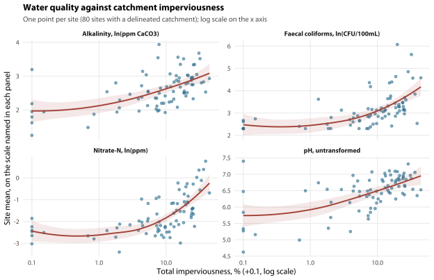
Only four parameters discriminate urban catchments at all, and three of them are laboratory measurements. Nitrate-N (rho = 0.68), faecal coliforms (0.69), pH (0.55) and alkalinity (0.58) all rise strongly with imperviousness. Conductivity (0.17), turbidity (0.16), temperature (0.05) and — surprisingly — phosphate (0.19) are effectively unrelated to it.
Alkalinity and pH rising with urbanisation is the concrete-and-mortar signature: Blue Mountains streams are naturally very soft and acidic (the desirable pH range is 5.28–6.75, which would be alarming almost anywhere else), and urban runoff over concrete raises both. It is a documented Sydney Basin pattern: Davies et al. (2010) reports the same alkalinity and pH elevation across urban streams in northern Sydney, against otherwise very soft reference water. Wright and Burgin (2009) records an elevation of the same kind in an upland sandstone catchment, but the discharges it studies are sewage effluent and coal-mine waste rather than urban runoff, and the full text could not be obtained to say which of them the elevation belongs to — so it corroborates the chemistry and not the mechanism argued here. pH is the odd one out: it tracks urbanisation far more strongly than any other probe parameter, though it is only fourth of the eleven on rank correlation, behind faecal coliforms, nitrate-N, and alkalinity — all of them laboratory measurements. It also has the weakest relationship with macroinvertebrate condition of any of the probe parameters (Section 6.6) — an urbanisation marker the animals barely respond to.
Phosphate’s near-zero correlation with imperviousness is the most interesting entry in Table 6.12, because phosphate is also one of the stronger individual water quality predictors of macroinvertebrate health (Section 6.6). Being clear about what it is: this is a null result, not a finding — rho = 0.19, q = 0.18, across 80 sites. At least three things would produce it: genuinely point-source phosphate that does not scale with impervious fraction; the 54% non-detect rate flattening the contrast between sites; or simply little real variation in phosphate between these catchments. Nothing here separates them. The point-source reading would be worth testing against the sewer asset layer, and that is a suggestion rather than a result — a null correlation is not evidence of a point source.
6.6 Water quality and macroinvertebrate health
6.6.1 Same-day associations
1,343 macroinvertebrate samples from 122 stream sites have a usable water quality sample taken at the same site on the same day — that is, a matched sample that actually carries a measurement — of which 934 carry all four core probe parameters. (Counting edge stream samples that carry a health score, matching on the calendar alone gives 1,393, but 50 of those point at a record with no measurement of any kind.) Sample sizes are quoted per parameter in Table 6.13, because they differ substantially. Each parameter is standardised, so the coefficient is the change in the 0–5 health score per standard deviation of that parameter.
Both models carry a site and a year random effect. The year effect matters more here than anywhere else in the chapter: a three-year site mean of a water quality parameter moves with calendar time, and so does the health score (chapter 5), so without a year term any parameter that drifts over the record acquires an association with health for free. Adding it forces the association to be identified from comparisons between sites within a year, which is the only thing this cross-sectional design can honestly claim to measure.
| Parameter | n | Spot reading | 3-year site mean | ΔAIC | Better predictor |
|---|---|---|---|---|---|
| Salinity (PSU) | 1,051 | -0.137 (-0.207 to -0.067) | -0.153 (-0.244 to -0.063) | -3.90 | Spot |
| Temperature (°C) | 1,330 | -0.104 (-0.144 to -0.063) | -0.125 (-0.177 to -0.074) | -2.54 | Spot |
| Conductivity (µS/cm) | 1,227 | -0.076 (-0.132 to -0.021) | -0.119 (-0.191 to -0.046) | +2.52 | Averaged |
| Turbidity (NTU) | 1,163 | -0.066 (-0.120 to -0.012) | -0.100 (-0.159 to -0.040) | +4.91 | Averaged |
| Faecal coliforms (CFU/100mL) | 968 | -0.053 (-0.096 to -0.011) | -0.095 (-0.149 to -0.041) | +5.28 | Averaged |
| Alkalinity (ppm CaCO3) | 1,213 | -0.087 (-0.138 to -0.036) | -0.077 (-0.138 to -0.015) | -5.27 | Spot |
| pH | 1,332 | -0.041 (-0.092 to 0.010) | -0.063 (-0.121 to -0.005) | +1.97 | Tie |
| Phosphate (ppm, as PO4 or as P) | 1,098 | -0.054 (-0.095 to -0.013) | -0.053 (-0.099 to -0.008) | -1.62 | Tie |
| Nitrate-N (ppm) | 994 | +0.032 (-0.019 to 0.083) | 0.000 (-0.064 to 0.065) | -1.51 | Tie |
| Dissolved oxygen (% sat.) | 1,198 | +0.103 (0.054 to 0.151) | +0.130 (0.071 to 0.188) | +1.71 | Tie |
| Dissolved oxygen (mg/L) | 1,290 | +0.110 (0.065 to 0.155) | +0.131 (0.079 to 0.183) | +1.57 | Tie |
6.6.2 Averaged conditions beat spot readings, for some parameters
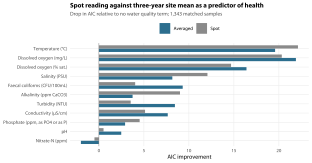
Averaging a site’s water quality over the preceding three years predicts macroinvertebrate condition better than the same-day reading for the parameters that reflect catchment loading. For faecal coliforms the AIC improvement rises from 4.0 to 9.3; for turbidity from 3.5 to 8.4. 3 of the eleven parameters are better predicted by the three-year mean — conductivity, turbidity, and faecal coliforms. Water temperature, salinity, and alkalinity are the exceptions, where the spot reading is the better predictor: they vary less within a site, so there is less for an average to remove.
The year random effect changes the size of this result, and phosphate is the clearest casualty. Treat every sample in a field round as an independent observation and the AIC improvements are several times larger, with phosphate the strongest predictor in the set (32.7 for the spot reading rising to 66.5 for the three-year mean). With the year effect in place phosphate’s advantage from averaging disappears entirely (4.5 and 2.9). That is not a technicality: most of what looked like a phosphate–health relationship was the two series drifting over calendar time together — which is the same problem Section 7.5 describes from the other side, since what drifted in the phosphate series was largely the detection rate. The parameters whose averaged advantage survives — conductivity, turbidity, and faecal coliforms — are the ones where the relationship is genuinely between sites rather than across years.
For the parameters that vary least within a site — water temperature, salinity, and alkalinity — the spot reading does as well or better, simply because there is less within-site variation for an average to remove. If water quality enters a health rating it should still enter as a multi-year site summary for all of them: the evidence here supports it for the loading parameters, and chapter 13’s reliability analysis supports it for the rest, because a single visit is a noisy draw whatever is being measured.
Keep the sizes in view. Set aside temperature and salinity, which the caveats below explain are not readable as water quality effects at all: the largest of the remaining averaged associations is dissolved oxygen (mg/L) at +0.131 points per standard deviation, which moves the health score by about an eighth of a score point. Water quality explains some of the difference between creeks. It does not explain most of it, and the methods document is right to warn against reading too much into a same-day correlation.
The faecal coliform row is the one to read with its window in mind. Its three-year averages start at 2006, like every other coliform quantity here, so 109 matched samples that carry a coliform result are set aside and the row is fitted on the remaining 968 — the smallest n in Table 6.13. That is what Section 3.7.6’s bench break costs here, and it is a cost in precision rather than in direction: the coefficient is -0.095 per standard deviation and clearly separated from zero, and coliforms gain more from averaging than any other parameter in the table.
Two of these associations need a caveat rather than a reading. Temperature is -0.125 points per standard deviation, but colder sites in this dataset are higher-altitude, headwater, less-disturbed sites: the coefficient is measuring altitude, not a thermal effect. Salinity is among the largest coefficients (-0.153), but it is the derived quantity whose conversion changed, and conductivity — the thing actually measured — gives a weaker association (-0.119). Neither belongs in a causal story.
6.6.3 Which parameters matter jointly?
Fitting eight of the eleven averaged parameters together (1,012 samples, 87 sites) separates the parameters that carry independent information from those that are merely correlated with the rest. The other three — water temperature, dissolved oxygen (% saturation), and salinity — are held out for the reasons given in the caption to Table 6.14, and nothing here tests them.
| Parameter | Estimate | 95% CI | Independent? |
|---|---|---|---|
| pH | -0.075 | -0.156 to 0.006 | No |
| Dissolved oxygen (mg/L) | +0.133 | 0.068 to 0.197 | Yes |
| Conductivity (µS/cm) | -0.010 | -0.097 to 0.078 | No |
| Turbidity (NTU) | -0.035 | -0.100 to 0.029 | No |
| Alkalinity (ppm CaCO3) | -0.125 | -0.199 to -0.052 | Yes |
| Phosphate (ppm, as PO4 or as P) | -0.045 | -0.092 to 0.002 | No |
| Nitrate-N (ppm) | +0.032 | -0.032 to 0.095 | No |
| Faecal coliforms (CFU/100mL) | -0.047 | -0.100 to 0.006 | No |
Only dissolved oxygen (mg/L) and alkalinity hold up when fitted together; pH, conductivity, turbidity, phosphate, nitrate-N, and faecal coliforms do not. The parameters that drop out are individually strong predictors but redundant once alkalinity is in the model — the between-site correlations among the laboratory parameters run from 0.3 to 0.6, so they are largely measuring the same underlying gradient of catchment disturbance.
Phosphate does not survive this model once year-level clustering is included. Its coefficient is -0.045 (-0.092 to 0.002); with a site random effect alone it is roughly two and a half times that size and comfortably significant. Alkalinity goes the other way — it is stronger with the year effect in place than without, because it is identified from differences between catchments rather than from drift over the record, which is exactly the property a scoring parameter needs. That contrast is the main reason Section 6.9 puts alkalinity first and phosphate on hold.
6.7 Flow state at the time of sampling
Almost every model in this chapter carries a residual that no measured covariate explains, and the obvious suspect has always been how much water was moving past the probe. The numeric ave_flow_m_s field is filled in on 558 of the 2,688 water quality visits, too few and too concentrated in recent years to enter a model. But the site description sheet has a free-text water_level box that officers have filled in on 1,005 visits since 2008, and it holds an ordered flow-state scale. Chapter 9 (Section 9.3.3) describes how it is recovered from the free text and normalised to six ordered levels. This section asks what it does to the water chemistry.
6.7.1 Flow state is not evenly distributed over the record
Before any of this is used to reinterpret anything, the confound has to be stated. The record looks at first as though flow state drifts upward — +0.48 scale points per decade (-0.16 to 1.11, p = 0.159, 912 samples at 83 sites, 2008–2025) — but that interval spans zero, and it should. There are 18 rounds here, and flow state swings more from one round to the next than the fitted change across the whole record. A steady rise is not what this is, and it should not be quoted from here as one. It is a block, and the block is what matters. Mean flow state is 2.92 under the Hydrolab, 2.66 under the Aquaread and 3.68 under the Aqua TROLL. The Aqua TROLL era is 2020 onwards, which in eastern Australia is the wettest run of years in the record (chapter 4). The instrument boundary at 2020 and the break in the weather are the same boundary, and flow state cannot separate them any more than the calendar can.
That cuts against the temptation to use flow to explain away the dissolved oxygen steps of Section 3.7.2, and it cuts the other way too: some of what those steps measure could be flow rather than probe. The rest of this section keeps season, linear trend and instrument era in every model, so the flow coefficients below are what survives all three.
6.7.2 What a step up the scale does
| Parameter | n | Unadjusted | Adjusted effect per level (95% CI) | p |
|---|---|---|---|---|
| Dissolved oxygen (mg/L) | 879 | +0.272* | +0.326 (0.249 to 0.402) | < 0.001 |
| Dissolved oxygen (% sat.) | 870 | +2.695* | +2.701 (1.947 to 3.454) | < 0.001 |
| Temperature (°C) | 902 | +0.020 | -0.191 (-0.310 to -0.073) | 0.002 |
| Nitrate-N (ppm) | 838 | +0.072* | +0.076 (0.014 to 0.138) | 0.016 |
| Faecal coliforms (CFU/100mL) | 842 | +0.113* | +0.099 (0.016 to 0.182) | 0.020 |
| Conductivity (µS/cm) | 873 | -0.020* | -0.020 (-0.038 to -0.002) | 0.026 |
| Phosphate (ppm, as PO4 or as P) | 839 | -0.076* | -0.068 (-0.131 to -0.005) | 0.035 |
| Turbidity (NTU) | 851 | +0.089* | +0.082 (-0.004 to 0.168) | 0.063 |
| pH | 905 | +0.017 | +0.026 (-0.004 to 0.056) | 0.086 |
| Salinity (PSU) | 878 | -0.009 | -0.008 (-0.027 to 0.011) | 0.424 |
| Alkalinity (ppm CaCO3) | 882 | +0.002 | -0.002 (-0.032 to 0.029) | 0.920 |
Flowing water is better-oxygenated water, and that is much the largest effect flow state has on anything you measure. Each step up the scale adds 2.70 percentage points of saturation (870 samples, p < 0.001) and 0.33 mg/L (p < 0.001). Across the full scale, from no flow to high, that is about 13.5 percentage points of saturation — a larger spread than anything else in this chapter accounts for at the level of a single visit.
This is physically unremarkable, which is the point: it is a sanity check the recovered field passes. Turbulent water equilibrates with the atmosphere and a stagnant pool does not, so oxygen saturation should track flow, and it does. Water temperature falls 0.19 °C per step once season is controlled, which is the same mechanism seen from the other side.
Below dissolved oxygen the effects are small and none of them would carry a recommendation on its own. Faecal coliforms rise +10% per step (p = 0.020) and nitrate-N +8% (p = 0.016), which is consistent with catchment washoff: the water that is moving is the water that has recently run off a surface. Conductivity falls -2% (p = 0.026), the dilution signature. Turbidity points up but does not clear 5% once season and era are controlled (p = 0.063), and pH does not move at all. Phosphate falls -7% (p = 0.035), which is reported for completeness and should not be interpreted: Section 7.5 shows that most of what the phosphate series measures is how often the test kit detected anything, and a change in detection frequency with flow would produce this coefficient with no change in the water.
The dissolved oxygen result is the only one here that is robust to how the scale is built. Two site-days carry two site descriptions recording different flow states, one of them an outright contradiction (moderate against no flow on the same sample code); the data layer sets both to NA rather than picking one. That choice moves nothing in Table 6.15 — the models above gain one sample and no p-value shifts in the third decimal place — but it is a reminder of how thin the sub-5% results are. Turbidity and phosphate sit either side of the 0.05 line and would swap places under a different but equally defensible handling of a handful of rows. Dissolved oxygen is nowhere near that boundary.
6.8 Climate
Chapter 4 established that the record runs from the tail of the Millennium Drought into the wettest years of the series. Turbidity, conductivity and the nutrients are all sensitive to antecedent rainfall, so the question is whether any trend is really a change in the weather.
| Parameter | Recent rain (7-day) | Wet/dry year (SPI-12) | Trend before climate | Trend after climate |
|---|---|---|---|---|
| Temperature (°C) | -0.009 | -0.148 | +0.581 | +0.616 |
| pH | +0.002 | +0.023 | -0.009 | -0.013 |
| Dissolved oxygen (% sat.) | +1.865* | -0.528 | +6.182 | +5.568 |
| Dissolved oxygen (mg/L) | +0.167* | +0.026 | +0.239 | +0.166 |
| Conductivity (µS/cm) | -0.011 | -0.080* | +0.130 | +0.148 |
| Salinity (PSU) | -0.016* | -0.017 | -0.162 | -0.149 |
| Turbidity (NTU) | +0.002 | +0.114 | -1.267 | -1.314 |
| Alkalinity (ppm CaCO3) | -0.030* | -0.059 | +0.069 | +0.075 |
| Phosphate (ppm, as PO4 or as P) | -0.031 | -0.001 | -0.437 | -0.414 |
| Nitrate-N (ppm) | -0.017 | -0.108 | -0.173 | -0.119 |
| Faecal coliforms (CFU/100mL) | +0.110* | +0.128* | -0.323 | -0.430 |
Two of the coefficients in Table 6.16 are worth putting in plain language.
- Faecal coliforms respond strongly to rain in the previous week (0.110 log units per e-fold increase, t = 3.5), which is what wash-off from an urban catchment looks like and is a reason to record antecedent rainfall on the field sheet.
- Turbidity is, if anything, higher in wet years (0.114 log units per unit of SPI-12, t = 1.5). SPI-12 takes one value per year, so with a year random effect in the model it is estimated from 27 effective observations, and only conductivity and faecal coliforms show a wet-year effect that clears the table’s own |t| > 2 — none of which carries a conclusion here. The direction still matters for the instrument argument: the record has become wetter, which if anything should have pushed turbidity up, and observed turbidity fell sharply. Climate therefore makes the apparent turbidity decline harder to explain environmentally, not easier.
Including climate does not materially change any trend estimate — the largest shift is for Dissolved oxygen (% sat.) — so no conclusion in this chapter rests on the drought breaking.
6.9 Is water quality fit to enter a health rating?
This section is the input to a decision made elsewhere. Chapter 15 (Section 15.3.6.1) adjudicates whether water quality should join the rating at all, weighing what follows against chapter 9’s finding that water quality separates creeks less well than the macroinvertebrates already do. What is settled here is the narrower and prior question: if water quality were to enter a rating, which parameters could carry the weight?
For each parameter Table 6.17 combines five things: how many sites carry it, how complete the record is, how heavily censored it is, whether it is exposed to the probe changes, and how strongly it relates to macroinvertebrate condition and to catchment imperviousness.
| Parameter | Type | Sites | Years | Cens. | Instrument-safe | Health assoc. | Imperv. rho |
|---|---|---|---|---|---|---|---|
| Temperature (°C) | Probe | 122 | 27 | – | Yes | -0.13* | 0.05 |
| pH | Probe | 122 | 27 | – | No | -0.06* | 0.55* |
| Dissolved oxygen (% sat.) | Probe | 117 | 26 | – | Yes | +0.13* | 0.11 |
| Dissolved oxygen (mg/L) | Probe | 121 | 27 | – | No | +0.13* | -0.03 |
| Conductivity (µS/cm) | Probe | 121 | 26 | 0% | No | -0.12* | 0.17 |
| Salinity (PSU) | Probe | 91 | 21 | <1% | No | -0.15* | 0.20 |
| Turbidity (NTU) | Probe | 122 | 25 | 23% | No | -0.10* | 0.16 |
| Alkalinity (ppm CaCO3) | Lab | 120 | 26 | <1% | n/a (lab) | -0.08* | 0.58* |
| Phosphate (ppm, as PO4 or as P) | Lab | 112 | 22 | 54% | n/a (lab) | -0.05* | 0.19 |
| Nitrate-N (ppm) | Lab | 89 | 19 | 5% | n/a (lab) | 0.00 | 0.68* |
| Faecal coliforms (CFU/100mL) | Lab | 87 | 20 | 47% | n/a (lab) | -0.10* | 0.69* |
| Parameter | Fit for a health rating? |
|---|---|
| Alkalinity (ppm CaCO3) | Yes — stable, complete, off the probe, independent |
| Conductivity (µS/cm) | Yes, secondary — steps at both probe changes, so score within an era; weak on health |
| Nitrate-N (ppm) | Yes, secondary — strongest imperviousness marker, from 2006 |
| Phosphate (ppm, as PO4 or as P) | Not yet — 54% non-detect and the kit history is undocumented |
| Dissolved oxygen (mg/L) | With caution — rebaseline at each probe change |
| Dissolved oxygen (% sat.) | No — duplicates DO (mg/L); its trend is absorbed by the era terms |
| Faecal coliforms (CFU/100mL) | Not yet — the 2004-05 break is unexplained |
| pH | No — unstable; weakest health signal of the probe parameters |
| Salinity (PSU) | No — derived from EC and the conversion changed |
| Temperature (°C) | No — a climate signal, not a condition signal |
| Turbidity (NTU) | No — probe-dependent and 23% censored |
6.9.1 The recommendation
Three parameters would make defensible components of a waterway health score: alkalinity, nitrate-N and conductivity, in that order — all three as a multi-year site mean rather than a spot reading (Table 6.18). Conductivity carries a condition the other two do not: it is the only one of the three on the probe, its level steps at both probe replacements, and it can therefore be scored only within an instrument era or against a baseline re-set at each changeover. Phosphate is held back until its test-kit history can be documented.
The reasoning, in short:
- Two of the three are laboratory measurements, so the probe replacements that dominate the rest of the record do not touch them. Whatever else changes, that is the property that makes a long series possible at all.
- Alkalinity carries independent information about macroinvertebrate condition when the eight jointly modelled parameters are fitted together (Section 6.6), and it is the only parameter that does so and is also scoreable: dissolved oxygen is on the probe and would need rebaselining at every changeover, and faecal coliforms carry the 2004–05 break. It is <1% censored, complete over 26 years at 120 sites, and — unlike phosphate — its association with health survives the year random effect rather than being erased by it.
- Nitrate-N is the strongest single marker of catchment imperviousness measured (rho = 0.68), which makes it the parameter most likely to register a change in catchment management. Its record is shorter — usable coverage begins in 2006 — and it is exposed to the 2017–2019 laboratory excursion, so it belongs as a secondary component rather than a headline one.
- Conductivity is a secondary physical measure, and it is the one of the three that comes with an instrument condition. It shows no detectable trend over 27 years, though the interval is wide (Section 6.4.3). What it is not is probe-independent: its level steps significantly at both probe replacements — +18% at 2017 and +30% at 2020 (Section 3.7.2) — so a conductivity series read straight across a changeover is reading the probe. That does not make it uninformative, and it is not a reason to drop it: a level shift at a known date is the one kind of instrument problem you can score around. It does mean conductivity can be scored only within an instrument era, or against a baseline re-set at each changeover, and that a card comparing 2016 with 2021 conductivity without that adjustment is not a comparison of water. Its relationship with health is weak and it does not track imperviousness, so it should carry less weight in any case — and it must also be scored within altitude zone, because lower-altitude streams run several times the conductivity of headwaters for reasons of geology alone.
Conductivity is not unusual in this respect, which is the wider point. Five of the seven probe parameters step significantly at at least one of the two replacements (Table 6.17). The probe record is the part of this dataset that most needs an overlap round (Section 3.8), and conductivity is recommended in spite of that rather than in ignorance of it.
Phosphate is the hardest call in this chapter. It is the strongest single predictor of macroinvertebrate health in the raw record, and on that alone it would be the first component of a score. Three things stop it:
- 54% of phosphate readings in the primary set are non-detects, so a mean is mostly a statement about detection frequency;
- the annual non-detect rate has swung between 9% and 90% between adjacent blocks of years, which is a kit history rather than a catchment (Section 7.5 has the detail, and it is worse than it looks in a report card);
- its independent contribution in the multivariable model does not survive year-level clustering (Section 6.6), and neither does its advantage from three-year averaging.
The detection limit is inferred, not confirmed. It is the grid the results were written on: no phosphate or nitrate-N value below 0.01 ppm exists in the raw record in any year, and where a sample carries a single reading the smallest positive value of either parameter is 0.01 ppm. The handful that sit under that grid — all 10 of them, 2012 only — are laboratory duplicates averaged rather than readings, so they are no evidence of a finer kit (Section 3.7.5). What the grid cannot tell us is the floor of the kit itself: a kit that could only see 0.1 ppm, writing its results onto this grid, would leave the same trace. Of everything this chapter asks you for, confirming which kit was used and what limit it states is worth the most, and it is probably an afternoon with the purchase orders. Phosphate becomes the strongest candidate in the set the moment that documentation exists. Until then we would leave it out of the score.
If phosphate has to be reported in the meantime, the statistic to use is the proportion of visits at which phosphate was detectable — not a mean, and not a pass rate against the trigger. It is what the pass rate is already measuring, it is immune to the substitution question entirely, and it is honest about the fact that a “pass” is usually a non-detection. Label it a property of the test, not of the water: its own association with macroinvertebrate health, once field rounds are treated as clusters, is -0.041 points per standard deviation (-0.084 to 0.002), which is not established. It is a reporting statistic, not a scoring one.
Five parameters would not make defensible components:
- Turbidity is 23% censored against a floor with no documentary basis at all (Section 3.7.5), the two Aqua TROLL units of the same probe model disagree with each other about how often it returns a value at the floor, and its apparent improvement over the record is largely a probe step (Section 3.7.2). A reasonable field observation and a poor score component.
- pH is unstable at the five-year timescale, steps at placebo cut points as readily as at real ones, and — decisively — has one of the weakest associations with macroinvertebrate health of any parameter measured — the weakest of the probe parameters, with only nitrate-N and phosphate closer to zero overall (-0.063 points per standard deviation on a five-point scale, carrying no independent information once the other parameters are in the model). It would add noise for the sake of a signal that is really urbanisation, measured better somewhere else.
- Salinity is a derived quantity whose derivation changed mid-record. Score conductivity, which is what the probe actually measures.
- Dissolved oxygen in per cent saturation is a near-duplicate of dissolved oxygen in mg/L — the same measurement expressed against temperature and pressure — and what looks like a trend in it is absorbed by the instrument-era terms. Two versions of one quantity in a composite score would weight it twice. Score the mg/L series, on the rebaselining condition above, and not both.
- Water temperature is rising, and that is the one real trend in the chapter — but it is a regional climate signal rather than a measure of catchment condition, and it is strongly driven by when in the year the sample was taken. It belongs in a climate indicator, not a health score.
Faecal coliforms are the near miss. They have the second-strongest relationship with imperviousness, an averaged association with health that survives the year random effect, and they are the parameter the public most readily understands. But 47% of counts sit below the detection limit and everything before the 2004–05 break is a different measurement (Section 3.7.6). Find out what changed at the bench, settle on one enumeration method and stay with it, and coliforms would be a strong addition. On the present record they are not scoreable.
6.10 What we can and cannot say
| Question | Answer | Confidence |
|---|---|---|
| Has water quality changed? | One parameter of eleven. Water temperature is rising by about half a degree per decade averaged over the year — but not at one rate: +0.34 °C per decade in the cooler half of the year and +0.99 in the warmer (interaction p = 0.0009), so the single figure is an average weighted by a sampling calendar that moved (Section 6.4.3); alkalinity and nitrate-N show no detectable trend; conductivity shows none either but its interval is too wide to be informative; faecal coliforms (since 2006) do carry a significant fitted decline, but 47% of their readings are non-detects substituted at the floor, so it is a property of that floor as much as of the creeks and must not be reported as a decline; the apparent changes in dissolved oxygen, turbidity, pH, salinity and phosphate cannot be separated from measurement changes. | High for the temperature rise and for the nulls; high that the DO and turbidity movements are the probe, because Section 3.7.2 finds no overlap at either changeover and so cannot separate probe from creek either way. The temperature point estimate is specification-sensitive — it is 0.58 °C per decade and is printed with its interval throughout, but a sentence written for a reader should quote about half a degree, not two decimal places. Moderate for any SINGLE decadal rate: the season-by-trend interaction is significant, both season-specific rates exclude zero, and the whole-year figure is an average over a seasonal mix that changed across the record (Section 6.4.3, Section 6.4.1). |
| Which are trustworthy for trend? | The four laboratory parameters, because the probe changes do not touch them — subject to the 2004-05 coliform break, the 2017-2019 nutrient excursion, and the non-detect rates of phosphate and faecal coliforms, which put the size of any trend in those two partly in the substituted floor. | High in principle; moderate in practice, because Section 3.7.6 and Section 3.7.2 both found their discontinuity in the data rather than in a record of it. |
| Are individual sites changing? | None. 0 of 648 site-parameter tests survive false discovery rate control over the whole family after seasonal and instrument correction; the smallest adjusted q-value is 0.10. | High. The unadjusted scan finds 16, and every large group in it traces to a change chapter 3 documents — the probe (Section 3.7.2) or the calendar (Section 3.7.1). |
| Does it explain bug health? | Weakly on the day, better averaged over three years. dissolved oxygen (mg/L) and alkalinity carry independent information; pH shows the weakest health signal of the probe parameters. | Moderate. These are associations across sites, not causal effects; the strongest is about an eighth of a score point per standard deviation, and they shrink substantially once each field round is treated as a cluster. |
| Is it the drought breaking? | No. Adding antecedent rainfall and SPI-12 changes no trend materially. The wet-year effects themselves are weakly determined, because SPI-12 takes one value per year and there are only 27 of them. Only conductivity and faecal coliforms clear |t| > 2 among the wet-year effects once the year is treated as the unit, and no trend in this chapter rests on them. | High for the conclusion; low for the size of any individual climate coefficient. |
| Should it enter the rating? | If it enters at all, three parameters (alkalinity, nitrate-N, conductivity), as multi-year site means, and not before an instrument-overlap protocol is in place (Section 3.8). Conductivity is the only one of the three on the probe and its level steps at both replacements, so it can be scored only within an instrument era or against a baseline re-set at each changeover. Phosphate is held back until its test-kit history is documented. Whether water quality should enter at all is chapter 15’s call (Section 15.3.6.1). | Moderate. The parameter choice is well supported; the weighting, and the prior question of whether to include water quality at all, are judgements the rating review has to make. |
6.11 Limitations of this chapter
Chapter 3 carries the limitations of the record. These are the limitations of what this chapter did with it.
The instrument corrections are estimated, not measured. The era terms here are a before-and-after comparison at each changeover, because there is no overlap period to calibrate against (Section 3.7.2). A parameter that genuinely changed at the same moment as the probe cannot be told apart from a probe step, and where that is the case neither reading can be preferred over the other. That is a stronger statement than “the correction is uncertain”.
Both laboratory discontinuities were found in the data, not documented. The 2004–05 coliform break and the 2017–2019 nutrient excursion are large, the same at every site, and shaped like something that happened at a bench rather than in a creek — but only the laboratory’s own records would say what changed. Section 3.7.6 lists what to ask for.
Most of the substituted detection floors are a choice we made, not a limit anyone measured. 7 parameters get a floor. 3 of them are laboratory detection limits the data layer carries, and only one of those — faecal coliforms at 10 CFU/100 mL — is confirmed from a document; phosphate and nitrate-N are inferred from the smallest positive value in the database. The other 4 — conductivity, salinity, turbidity and alkalinity — have no documentary basis at all (Section 3.7.5). Alkalinity is the awkward one: the data layer looked at it and declined to infer a limit, and we substituted anyway. Every level trend for turbidity, phosphate and faecal coliforms is conditional on that choice; for conductivity and salinity the floor binds on less than a quarter of one per cent of readings, so it makes no difference.
A censoring-aware regional trend test has not been run. The Mann-Kendall cross-check runs on residuals, which destroys the ties non-detects would otherwise create, so for phosphate, faecal coliforms and turbidity it is not the censoring-robust test it is usually taken to be (Section 6.4.4). A proper censored-data model (Akritas–Theil–Sen, Tobit,
NADA::cenfit) needs confirmed detection limits, which do not exist for these data yet. The methods and worked R examples are in Helsel (2012) and in sections 5.5, 7.9 and 12.7 of Helsel et al. (2020), which is open access — the 2020 edition distributes censored-data methods through the book rather than collecting them in one chapter. This is the analysis to run the day the detection limits are confirmed.Everything annual is estimated from 27 observations. One round a year for 27 years is 27 observations of anything that varies annually — the era terms, SPI-12, any change of slope. Over a six-year window a step and a trend are nearly the same regressor, so once each year is allowed its own level almost no individual step is established. That is a limit of the monitoring design, not of the analysis.
718 of 2,688 water quality samples carry no measurement of any kind. They are recorded visits with no results. Whether the results were never taken, never entered or lost is not something this chapter can determine.
Replicate probe readings are averaged before the chapter sees them. 821 sample codes carry two to seven readings minutes apart, and the data layer averages them. That is the right choice for a level, but it discards a direct measure of within-visit measurement error — which is exactly the quantity several arguments here would have benefited from.
The health associations are cross-sectional. Sites with high phosphate are sites in urbanised catchments, and urbanised catchments differ in many ways besides phosphate. Nothing here identifies a causal effect of water quality on macroinvertebrates, and three-year averaging improves prediction without changing that.
The spatial analysis runs on 80 of the 122 stream sites — those carrying both a delineated catchment and at least five samples — and those are the sites of the modern network. The spatial analysis in Section 6.5 therefore describes the current monitoring set rather than the whole record. (Imperviousness itself is delineated for more than that; the binding filter here is the five-sample minimum, not the catchment layer.)
Whether the plateau chapter 5 finds in waterway health has a water quality counterpart is not settled here. The natural test is a change of slope at chapter 5’s estimated changepoint (Section 5.5.2), and the only series that moves enough to bend is the exceedance rate, which is chapter 7’s (Section 7.4). On this chapter’s level trends there is nothing to test against, because ten of the eleven have no established trend in the first place. So this chapter answers chapter 5’s question with “not from here”, which is not the same as “no”.
One family of tests here is corrected for multiplicity and the others are not. The site-level scan of Section 6.5 is a scan in the strict sense — 648 tests run in order to find which of them are significant — and the false discovery rate is controlled over it, both as one family and within each parameter. Nothing else is corrected: not the eleven parameter-level trends of Section 6.4.3, the 44 instrument step tests, the 33 regional Kendall tests published in three p-value forms each, the 22 spot and averaged association verdicts of Section 6.6, or the 22 rainfall and wet-year coefficients of Section 6.8, each of which carries its own |t| > 2 flag. Those are pre-specified sets, fixed before any of them was fitted and reported in full whether they clear anything or not, which is a different object from a scan and is why they are not treated as one — Section 3.7.2’s multiplicity caveat makes the same distinction for chapter 3 and says what is used there in place of a correction. What the decision costs, measured: six of the eleven parameter-level intervals exclude zero and five of them survive Benjamini–Hochberg over the eleven. The one that does not is phosphate, whose interval only just excludes zero — and Table 6.6 has already disqualified it for a better reason than a q-value (No — laboratory excursion at 2017-19), so correcting the eleven would change no verdict in this chapter and would not touch water temperature. As in chapter 3, that is a control on the family and not on any one row of it: a single interval lifted out of Table 6.6 on its own carries no protection at all.
| Item | Value |
|---|---|
| Data layer built | 2026-08-30 12:56 |
| R version | R version 4.4.3 (2025-02-28) |
| Primary analysis set | 1,304 samples, 122 sites, 1998-2025 |
| Matched macroinvertebrate samples | 1,343 samples, 122 sites |
| Model fits | read from the targets graph in R/_targets.R |