| Question | Answer | How much weight it bears |
|---|---|---|
| What most influences community composition? | Physical habitat, which uniquely explains 7.9% of compositional variation, ahead of water quality (3.8%), geography (1.7%) and catchment imperviousness (0.5%). Between creeks, imperviousness is the strongest single driver at 13%. | High for the ordering, which survives a site-level noise control, a metric embedding, year-detrending and a second design (Section 9.4.1, Section 9.4.2, Section 9.5). Low for the magnitudes: they depend on which sites have complete data, Section 9.4.2 shows they are an upper bound, and Section 9.4.1 shows that 54% of the habitat share and 60% of the water quality share is what random columns of the same width earn. Do not quote a unique share as an effect size. |
| How much does that close chapter 8’s gap? | The two new blocks raise explained variation from 19% to 31% on the same samples, closing about 15% of what was unexplained — 8.6% on a metric embedding of the same distance. Measured site variables now account for 72% of everything that separates one creek from another. | High for the comparison, which is on identical samples with identical methods; the absolute percentages are an upper bound. |
| Does imperviousness act directly, or through something? | Not answerable from a partition, but the water chemistry block is the one that behaves as though it is on the path. Imperviousness keeps 3.6% to itself in the four-block model and 0.5% in the six-block one, while fitted alone it still takes 6.1%. Replacing each added block with site-level noise of the same size leaves it 2.94% against 2.81% for real physical habitat, and 2.96% against 0.82% for real water quality. | Low for habitat, moderate for chemistry. A partition cannot prove a pathway, and the habitat block absorbs no more than random columns of the same shape do (Section 9.4.3). |
| Which levers can we actually pull? | Imperviousness first, and only indirectly. Of the reach-scale levers riparian shading is the strongest — 5.0% alone, rank 13 of 27 overall, unique contribution 1.2% — followed by trailing bank vegetation. Fine sediment (p = 0.127), sedimentation as recorded, and phosphate as a site mean do not rank at all. | Moderate. These are associations across creeks, not the results of an intervention — and shading is a state, not a trend (Section 9.3.2). |
| What moves a creek between visits? | Almost nothing measurable: 9.0% of within-creek variation, of which the largest single variable is sampling effort. The design would have detected any single variable above about 0.4%. Flow state, the driver most often nominated as the missing one, is now measured and takes 1.7% of within-creek variation on its own. | High, and it is a limit of the data rather than of the analysis, because the leading alternative explanation has now been tested rather than assumed. |
9 Why the creeks differ from one another
Blue Mountains City Council Healthy Waterways — statistical analysis
9.1 What this chapter answers
You asked which water quality and physical site characteristics most influence community composition. This chapter answers that one. The companion question — what is special about the sites that support the rarer families — is chapter 10, because it turned into a conservation argument rather than a driver ranking.
Chapter 8 partitioned compositional variation across four blocks — time, imperviousness, geography and climate — and left most of it unexplained. It named two blocks it had not tested: water quality, and physical habitat. This chapter tests both. The habitat block comes from tblSiteDescription: the shading, substrate, channel and vegetation records your field officers have written on every water quality visit since 2006, and which no analysis had previously used.
Four findings, in the order in which they should change what you do.
Physical habitat is the largest measured influence on community composition — larger than water quality, larger than imperviousness, larger than the passage of time. It uniquely explains 7.9% of compositional variation, against 3.8% for water quality, 0.5% for catchment imperviousness and 2.8% for time (Section 9.4). That is an ordering, not a set of effect sizes — about 54% of the habitat figure and 60% of the water quality figure is what site-level columns of the same width earn from random numbers, and Section 9.4.1 gives the baseline for every block. The ordering survives that control; the sizes are upper bounds twice over, here and at Section 9.4.2. Habitat is also the block measured least well, and Section 9.3.2 says how much that costs.
Imperviousness has almost nothing left of its own once chemistry and habitat are in the model — and only the chemistry half of that survives a control. Its unique share falls from 3.6% to 0.5% when the two new blocks go in (Section 9.4.3). But swap the habitat block for 13 columns of random numbers, one drawn per creek, and imperviousness is left with 2.94% — against 2.81% for the real thing. The habitat block does what noise of the same shape does. The water quality block does not: 0.82% real against 2.96% for noise. So sealed catchments and shifted chemistry go together more tightly than the arithmetic explains, and for habitat this design cannot say.
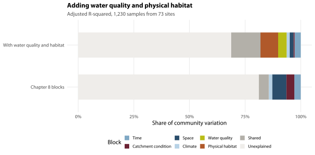
Together the two new blocks close about 15% of the gap chapter 8 left open, and the measured site variables now account for 72% of everything that separates one creek from another — we can largely say why Blue Mountains creeks differ. Read the magnitudes as an upper bound: Section 9.4.2 halves them and leaves the ordering intact. Of the things you can act on, imperviousness ranks first, and riparian shading is the strongest reach-scale lever (Section 9.5).
Within a creek, almost nothing measured predicts anything — including flow, which used to be the excuse. Everything recorded explains 9.0% of the difference between one visit and the next, and the largest single variable is how many animals were counted. The design would have found anything above about 0.4%, so this is a bound and not merely a null (Section 9.6). Flow state, recovered from the field sheet and tested here for the first time on 921 samples, moves composition significantly and moves it by 1.7% (Section 9.6.1). The driver everyone nominated as missing has been found and it is small.
9.1.1 What this chapter will and will not bear
9.2 The data behind this chapter
Each question and request below is set out again in What we need from you, with what it blocks, what an answer is worth and what it would cost you to find, ranked against every other ask in the report.
9.2.1 What this chapter uses, and where it came from
The block that comes out on top in this chapter is built entirely from tblSiteDescription — shading, substrate, macrophytes, riparian structure and riffle percentage — recorded by your field officers on about 1,100 water quality visits since 2006, and never analysed before.
Thirteen variables, reduced to a site mean wherever a site has at least two descriptions. Substrate is eight percentages that do not always sum to 100; a description is used only where at least six classes are recorded and the total falls between 50 and 200, and it is then renormalised to proportions. Three derived summaries come out of it — a coarseness index (the cover-weighted mean of log10 nominal particle size), the percentage of fine sediment and the percentage of bedrock. Filamentous algae and periphyton are recorded on too few descriptions to use.
Blocks: Nothing — this is a statement of what we used. Value: moderate. Costs you: minutes. Refer to it as
dq:habitat-block-provenance.
The imperviousness variable in this chapter is total catchment imperviousness, built in chapter 4 from road-corridor polygons and address points rather than measured, and entered on a square-root scale.
Worth knowing for two reasons. It is good enough to rank creeks against each other and not good enough to set a threshold on, which is chapter 4’s conclusion and this chapter inherits it. And it is not the connected (“DCI”) figure some earlier material used: total is about 2.78 times larger, though the two rank the catchments identically, so nothing in the ranking below turns on which one is used.
Blocks: Nothing — this is a statement of what we used. Value: moderate. Costs you: minutes. Refer to it as
dq:imperviousness-is-modelled-ch9.
9.2.2 What is wrong with it
About a quarter of the macroinvertebrate samples were taken before anyone wrote a site description, so those samples are being given habitat values measured years later.
The site means are unweighted averages over whatever descriptions a site happens to have, so a sample from 2001 is scored on a reach as it was described from 2006 onward. We have tested what it costs: restricting the partition to the period the descriptions actually cover raises habitat’s share rather than lowering it, so the backfill dilutes the finding rather than manufacturing it. There is no fix available in the data; it is a limit on how far back the habitat block can be read.
Blocks: Reading the habitat ranking back before 2006. Value: moderate. Costs you: minutes. Refer to it as
dq:habitat-backfill-pre-2006.
9.2.3 Questions only you can answer
The water quality sheet has an average flow velocity field filled in on about 558 visits. Was that ever measured with a meter, or is it an eye estimate — and if there was a meter, which one and over what years?
We ended up using the free-text water_level box instead, because it has nearly twice the coverage. But a velocity in metres per second, if it is a real measurement, is a better variable than a six-level ordinal judgement, and 558 visits is not nothing. If it was measured, it is worth going back for; if it was estimated by eye, we should say so and stop treating the units as meaningful.
Refer to it as
dq:ave-flow-provenance.
Does WaterNSW, Sydney Water, NPWS or a university hold a continuous flow gauge inside or near the monitoring network — and if so, can you tell us who to ask for the record?
Flow state recovered from the field sheets carries the level at the moment of sampling and structurally cannot carry antecedent discharge, time since the last flushing flow, or rising-versus-falling limb. Those three are what a gauge adds. Samples taken after rain score lower — 0.042 lower per e-fold of 30-day rainfall — and the recovered flow state does not absorb that, which is the clearest sign something hydrological is missing.
Refer to it as
dq:stream-gauges.
9.2.4 What would answer them
Would you apply for the full-resolution SEED Greater Sydney tree canopy layers (2016, 2019 and 2022)? It needs an application form and a signed NSW Digital Data Deed Poll, and Council is eligible as a Greater Sydney council.
It is the only remaining route to a network-wide canopy trend. SEED carries the near-infrared band that separates eucalypt canopy from everything else; the Nearmap RGB imagery we have does not, and excess-green calls 1.4% of a closed-canopy tile vegetation. Three epochs is the one thing that could still corroborate or kill the recorded shading trend.
Refer to it as
dq:seed-canopy-deed-poll.
9.3 The analysis sets, and why there are two
Every block is available for a different subset of samples, and the intersection is what carries the full model.
| Set | Samples | Sites |
|---|---|---|
| Edge stream macroinvertebrate samples | 1,502 | 125 |
| with a delineated catchment (imperviousness) | 1,454 | 117 |
| with site-level water quality (3 or more readings per parameter) | 1,259 | 76 |
| with site-level physical habitat (2 or more descriptions) | 1,271 | 78 |
| all blocks present (the analysis set) | 1,230 | 73 |
Chapter 8’s central warning governs everything here: creek identity alone takes over 40% of compositional variation, so any analysis that fits a site-level predictor to sample-level data without accounting for creek identity will credit the creek’s differences to whichever site variable happens to correlate with it. Two designs handle this honestly (Table 9.3).
| Design | Unit | Question it answers |
|---|---|---|
| Between-site | One averaged community per site | Why do creeks differ from one another? |
| Within-site | One sample, creek identity partialled out | What moves a creek’s community from visit to visit? |
The sample-level partition in Section 9.4 is reported first because it is the direct extension of chapter 8 and is comparable with it, but it inherits that chapter’s confound: site-level blocks in a sample-level analysis are explaining between-creek variation. Section 9.5 and Section 9.6 take that apart.
One number matters before anyone plans around a same-day design. Of the 1,502 edge stream samples here, 1,343 from 122 sites carry a same-day water quality sample that actually holds a measurement — wq_match_usable, not wq_match, which is only a statement about the calendar and is 1,392 over this same set. Within that set the per-parameter counts are 1,098 phosphate, 1,213 alkalinity, 994 nitrate-N and 1,227 conductivity, and only 868 samples carry all four at once. A four-parameter same-day block is that big, and no bigger.
9.3.1 What the laboratory and instrument breaks cost this chapter
Chapter 3 establishes three discontinuities in the water quality record that are measurement rather than environment. Every water quality variable here is built to respect them, and each one costs readings:
- Faecal coliforms step by about a hundredfold somewhere in the sampling gap between May 2004 and February 2005 (Section 3.7.6). Everything before 2006 is dropped, which is chapter 6’s cut and now ours: 98 results.
- Phosphate and nitrate reagents changed over 2017–2019 — the share of phosphate results below the detection limit fell sharply and then returned (Section 3.7.2). 183 nutrient results from those three years are dropped. ⚠ Phosphate also carries something that is not a break, cannot be dropped, and survives every filter in this chapter: its species is unconfirmed. Nothing in either database or the methods document says whether the readings are phosphate as PO4 or as P, and the two differ by a factor of three (Section 7.5,
dq:phosphate-units). Every phosphate quantity here is a count, a share, a p-value or a variance explained, all of them taken from that one column, so the ambiguity cancels out of them — but nitrate-N declares its species in its name and phosphate does not, so any phosphate concentration in ppm that leaves this report carries it. - The probe was replaced in 2017 and again in 2020. pH, dissolved oxygen, conductivity and turbidity lose no readings; they are centred within instrument era before averaging. That removes the step in level between one probe and the next. It does not touch the difference in spread, and for turbidity the spread does differ between eras by about a factor of two, so a site read mostly on one instrument has its deviations compressed relative to a site read mostly on another. Standardising within era — centring and scaling — rather than centring alone was tried, and it moves nothing this chapter uses: the two sets of site means agree closely and turbidity’s between-creek result is the same on either (Section 9.5, where it is the one variable on the 5% boundary in any case). The correction is a location shift and this bullet says so; it used to say the eras were made “comparable”, which claimed the scale as well.
The physical plausibility screen runs in the data layer before wq is built, so nothing further needed removing here. It is re-run above as a guard, where it removes nothing.
9.3.2 Physical habitat: what was recorded, and how well
The habitat block is the one this chapter ranks first, so its provenance matters more than any other block’s.
site_description holds 1,101 descriptions — shading, substrate composition, macrophytes, riparian structure, pool and riffle percentages — linked to water quality samples. 1,006 of them are stream sites, spanning 2006 to 2025 at 88 sites. Filamentous algae and periphyton are recorded on only 92 descriptions and are dropped.
The substrate percentages should sum to about 100 and often do not: of the 1,066 descriptions with any substrate recorded, 113 (10.6%) miss 100 by more than five points. Here, 933 of 1,006 descriptions record at least six of the eight classes with a total between 50 and 200 and are renormalised to proportions; the rest are set missing rather than analysed as recorded. 32 sample codes carry more than one description row, so a join from wq to site_description is one-to-many and has to be aggregated first.
| Variable | Site descriptions | Sites |
|---|---|---|
| Riparian shading (%) | 894 | 78 |
| Trailing vegetation (%) | 967 | 80 |
| Bank overhang (%) | 969 | 80 |
| Riffle (%) | 910 | 78 |
| Moss cover (%) | 958 | 79 |
| Macrophyte cover (%) | 909 | 80 |
| Sedimentation (%) | 886 | 80 |
| Detritus cover (%) | 961 | 80 |
| Algal cover (%) | 908 | 78 |
| Channel width (m) | 853 | 79 |
| Substrate coarseness | 933 | 80 |
| Fine sediment (% silt and clay) | 933 | 80 |
| Bedrock (% of substrate) | 933 | 80 |
These are estimates made by eye, by different officers, over 19 years, with no written protocol — and the block built from them still ranks first. That is uncomfortable enough to state up front rather than bury in a limitation. Section 3.6.2 diagnoses it in full — most of the 13 variables of Table 9.4 drift measurably within a fixed site, and on the descriptions that name a field officer, who wrote the sheet accounts for more of the variance than which creek it was on some of them. We are not going to re-derive any of that here; two chapters fitting the same model is how a number starts drifting.
Two tests say the ranking survives anyway, and they are the reason the block is kept. Rebuilding every site mean from year-detrended values and refitting the identical partition moves habitat’s unique share from 7.9% to 7.9% — so the primacy is not an artefact of drift. And 25% of the community record predates the first site description, meaning those samples carry habitat values measured later; restricting the partition to the period the descriptions actually cover raises habitat’s share to 9.3% on 1,058 samples. The backfill dilutes the finding rather than manufacturing it.
What does not survive is the direction of travel in riparian shading. The field record has shading rising, and Nearmap imagery says the creeks have not changed:
Within a single capture, a reach the officers called more shaded really is greener from above (+0.0129 SD of canopy per point of recorded shading, 95% CI 0.0086 to 0.0172, 325 site-captures) — the variable measures something real about a reach. Within a site, a year in which more shading was recorded is not a year in which the canopy was above that site’s own average (+0.0006 SD per point, 95% CI -0.0036 to 0.0048, 318 site-captures at 55 sites). So use shading as a state, and do not read a rise in it as improvement. That constraint travels with every recommendation in this chapter that mentions shading, and chapter 15 refuses shading as a rating factor partly on the strength of it.
The cheap fix is the obvious one and it is worth doing before the next season: a page of worked examples, photo points at each site, and the officer’s name on every sheet.
9.3.3 Flow state, recovered from a free-text box
The site description sheet also carries water_level, a free-text box recording how much water was moving past the officer at the moment of sampling. It is populated on 1,005 of the 1,101 descriptions, from 2008 to 2025. That is nearly twice the coverage of the numeric ave_flow_m_s field on the water quality sheet, which is filled in on 558 visits, and it is the reason flow state can now be analysed at all.
Because it is free text, the same handful of states had been entered thirteen different ways — moderate and mod, low and low flow, low/moderate and low-moderate and low-mod, mod/high and moderate-high, alongside no flow, high and two entries that are neither. The data layer parses the string rather than looking it up in a table of the spellings that happen to exist today: dl_normalise_flow() searches for the four base tokens (no flow, low, moderate, high), returns that level where exactly one is found, and returns the intermediate level where exactly two are found that bracket one — low with moderate, or moderate with high. The result is flow_state, an ordered factor on the six-level scale no flow < low < low-moderate < moderate < moderate-high < high, and flow_level, the same thing as an integer for modelling. The raw string survives as water_level.
A parser rather than a lookup because a lookup fails silently. The fourteenth spelling typed into the box next year returns NA from a lookup table and the series quietly shrinks by one; here it either resolves, because it is built from the same four words, or it is refused and listed in dl_issues. Anything appearing in that list is a spelling the normaliser should be taught, not a data error to shrug at.
1,003 of the 1,005 populated entries normalise; the two that do not are left NA deliberately, and they are n/a and no flow- moderate. The first is an explicit non-observation. The second names two states three steps apart on a six-point scale, with no defined midpoint between them; assigning it a level would be inventing an observation rather than reading one.
Flow state is a property of the visit, not of the water quality sample code, so site_flow reduces it to one row per site-day. That is what makes it joinable to macroinvertebrate samples, which share no sample code with the water quality database, and it is why more water quality samples carry a flow state (1,038) than there are populated water_level records: one description covers every sample taken at that site that day. flow_state and flow_level are carried on wq and on bug_wq (997 macroinvertebrate samples). Two site-days whose two descriptions record different flow states are set to NA rather than arbitrated.
The same sheet’s weather field had sunny and Sunny — and sunny with a trailing space — stored and counted as three values rather than one. weather is now case-folded and squished, which collapses 9 raw spellings to 5; weather_raw keeps what was typed. No semantic tidy has been attempted, so sunny & windy and partly cloudy remain distinct from sunny and cloudy.
9.4 How much of the unexplained variation do the new blocks close?
Chapter 8’s four blocks are refitted here on exactly these samples, so the before-and-after comparison is not confounded with a change of sample set. Every “chapter 8’s four blocks” figure below is this refit, not a number carried over from that chapter.
The tool is variance partitioning on a distance-based redundancy analysis: each block of variables is fitted to the community dissimilarity matrix, and the overlaps between blocks are resolved so that each block’s unique contribution is what it explains that no other block can (Legendre and Anderson 1999). The percentages reported are adjusted R-squared rather than raw, because the raw value rises whenever a variable is added whether or not it explains anything, and the adjusted form is the one Peres-Neto et al. (2006) show to be unbiased for RDA — including Hellinger-based db-RDA — with two equal-sized predictor blocks. They do not test Bray–Curtis db-RDA, and name it as a case their assessment did not cover; nor do they test blocks of unequal size, which is the situation here, since the six blocks hold very different numbers of variables. So the adjustment is the right correction to reach for and it is not one this design has external warrant for — which is one more reason Section 9.4.2’s reading is the operative one: the ordering holds, the magnitudes do not.
| Block | Alone | Unique |
|---|---|---|
| Time | 3.2% | 2.8% |
| Catchment condition | 6.1% | 0.5% |
| Space | 9.7% | 1.7% |
| Climate | 5.4% | 1.4% |
| Water quality | 13% | 3.8% |
| Physical habitat | 16% | 7.9% |
| Shared between blocks | 13% | |
| Explained in total | 31% | |
| Unexplained | 69% |
Physical habitat is the largest single measured influence on community composition. It uniquely explains 7.9% of compositional variation — more than water quality (3.8%), more than geography (1.7%), more than time (2.8%) and more than catchment imperviousness (0.5%). Read that as an ordering and not as a set of effect sizes. A block of site-level columns earns a share of this partition whether or not it explains anything, and Section 9.4.1 measures how much: about 4.3% of habitat’s 7.9% is what 13 columns of random numbers would take. The ordering survives that control. Imperviousness’s 0.5% is small enough that the control cannot resolve it either way, and Section 9.4.3 is where that gets taken apart.
The comparison that matters for the monitoring program is with chapter 8. Fitted to these same 1,230 samples, chapter 8’s four blocks explain 19% and leave 81% unexplained. Adding water quality and physical habitat raises the explained share to 31%, a gain of 12%. The two new blocks close about 15% of the gap chapter 8 left open, and they roughly 1.6-fold the explanatory power of the whole exercise.
9.4.1 What a block of this size would earn from random numbers
A second caveat belongs to the same numbers, and it is the larger of the two.
There are 1,230 samples in this partition but only 73 creeks, and the habitat and water quality blocks are site means — one value per creek, repeated across every sample from that creek. Section 9.4.3 states that arithmetic exactly, and runs a control for it. But it runs the control on one variable, imperviousness, and the same arithmetic applies with equal force to each block’s own unique share — which is where the numbers above live. The adjusted R-squared is meant to protect against precisely this, and Peres-Neto et al. (2006) is cited above for that reason; but their correction counts sample-level degrees of freedom, and on 1,230 rows carrying 73 independent values it is calibrated against the wrong n.
So run Section 9.4.3’s placebo against the blocks themselves. Replace each block with the same number of columns of site-level noise — one number drawn per creek, repeated across that creek’s samples — and refit the identical partition, 20 draws each. Noise cannot explain composition, so whatever it takes is what the design hands a block of that width for nothing.
| Block | Variables | Published unique share | The same width of noise | Net of noise | p |
|---|---|---|---|---|---|
| Physical habitat | 13 | 7.9% | 4.3% (3.2% to 5.3%) | 3.6% | 0.048 |
| Water quality | 8 | 3.8% | 2.3% (1.4% to 3.6%) | 1.5% | 0.048 |
| Space | 3 | 1.7% | 0.7% (0.4% to 1.0%) | 1.0% | 0.048 |
| Catchment condition | 1 | 0.5% | 0.2% (0.1% to 0.4%) | 0.3% | 0.048 |
The ordering survives the control. The magnitudes do not, and one comparison fails outright. Physical habitat stays the largest measured block on either reading — 7.9% against water quality’s 3.8% as published, and 3.6% against 1.5% net of its own null — so “the largest single measured influence” holds. But 54% of the published habitat figure and 60% of the published water quality figure is reproduced by random numbers, and the baseline scales with the width of the block: 13 columns of nothing earn 4.3%, 8 earn 2.3%, 3 earn 0.7% and 1 earns 0.2%. So a unique share in Table 9.5 is not an effect size, and two blocks of different widths are not comparable on it without their baselines.
The comparison that fails is imperviousness, and it fails by being unresolvable rather than by being refuted. Catchment condition enters the partition as a single column, and a single column of noise earns 0.2% against its published 0.5% — a gap of about two to one, on a quantity so small that the draws straddle it. On the 20 draws tabulated here none reached the published value; on an independent set of 20 one did. One draw in forty is not a result in either direction. So the honest statement is that at this sample size the design cannot separate imperviousness’s unique share from what a column of nothing would earn — not that it has none, and not that it has one.
That is enough to withdraw one sentence and to sharpen another. The chapter cannot say that physical habitat explains an order of magnitude more composition than imperviousness does; a ratio of two numbers is meaningless when the smaller one is inside its own noise. And it does not need to: the reason imperviousness has almost nothing left of its own is the one Section 9.4.3 spends a page on — with 73 creeks it is very largely a linear combination of the habitat and chemistry site means (R-squared 0.77) — and that argument does not depend on this p-value at all.
What the limitation costs, plainly. Three things, and none of them is recoverable by reanalysing these data.
- No percentage in Table 9.5 can be quoted as an effect size, here or anywhere downstream, without the baseline beside it. The summary figure 7.9% travels into other chapters; 4.3% has to travel with it.
- Blocks of different widths cannot be ranked by how much more they explain, only by whether they explain more. “Habitat is roughly twice water quality” survives net of noise (3.6% against 1.5%); “habitat beats imperviousness 17-fold” does not, and is withdrawn.
- A recommendation resting on this partition rests on its ordering. That is what R10 — a riparian and geomorphic rapid assessment as a third reporting panel — is entitled to, and the ordering is unusually robust: it survives this control, it survives the metric embedding of Section 9.4.2, it survives year-detrending and the 2006-onward restriction (Section 9.3.2), and the between-creek ranking of Section 9.5 reaches the same place by a design that does not have this problem at all. What R10 is not entitled to is the size of the gap.
None of that is a reanalysis waiting to be done. The baseline in Table 9.6 is fitted rather than quoted — ch09_block_placebo() runs Section 9.4.3’s placebo against each block’s own unique share on 20 draws, and both sides of every comparison in the table move together on a refit — so the limitation is a property of the design and the sample size, not of the arithmetic.
9.4.2 The percentages are inflated; the ordering is not
One caveat has to be attached to every number in this section, once, plainly. Bray–Curtis distances are not Euclidean, so the ordination embeds the samples in a space that has imaginary axes as well as real ones. This is a known property of the method rather than a fault in the data: Legendre and Anderson (1999) set it out when they introduced distance-based redundancy analysis, and report that taking the square root of a Bray–Curtis distance removes the negative eigenvalues in practice — a result they attribute to unpublished simulations and note is not proven, though the corresponding result for the binary form (Sørensen) is. The property at stake is being Euclidean, not merely metric. That is the correction applied below, and it is standard; but it is an acknowledged conjecture rather than a theorem, which is one more reason to read this section for its ordering rather than its magnitudes. Here 922 of the 1,229 eigenvalues are negative and they carry 23% of the total absolute eigenvalue mass. Because those negative values are subtracted from the total inertia that every adjusted R-squared above is divided by, the denominator is smaller than the real variation in the data and every percentage in this section is inflated by roughly 1.7 times.
Refitting the identical partition on the square root of the same distance, which removes the negative eigenvalues, gives the honest magnitudes:
| Block | Bray-Curtis | Square-root (metric) |
|---|---|---|
| Time | 2.8% | 1.5% |
| Catchment condition | 0.5% | 0.3% |
| Space | 1.7% | 1.1% |
| Climate | 1.4% | 0.8% |
| Water quality | 3.8% | 2.4% |
| Physical habitat | 7.9% | 4.9% |
| Chapter 8’s four blocks together | 19% | 10.6% |
| All six blocks together | 31% | 18.3% |
| Share of the gap closed | 15% | 8.6% |
The ordering is robust and the absolute percentages are not. Physical habitat still leads, still ahead of water quality, time, geography, climate and imperviousness, in the same order. But “explained variation rises from 19% to 31%” should be read as “from 10.6% to 18.3% of the real compositional variation”, and the share of chapter 8’s gap that the two new blocks close is 8.6%, not 15% (Table 9.7). Ratios between blocks in this chapter are trustworthy; the percentages themselves are an upper bound.
9.4.3 What imperviousness works through
This gets its own section, because it is where the partition is easiest to over-read.
The unique fraction for catchment imperviousness falls when the new blocks go in — from 3.6% in the four-block model to 0.5% in the six-block one — and the same happens to geography (6.3% to 1.7%). Fitted on its own, imperviousness still explains 6.1%, so nothing about it has become less important. The tempting reading is that its effect has been given a mechanism — that the part which used to be unique to imperviousness is now shared with habitat and chemistry because those are the things a sealed catchment acts through.
The tempting reading is half right, and it is worth spending a page on which half, because the other half is arithmetic.
Start with what the arithmetic can do on its own. Across the 73 creeks in this set, imperviousness is very largely a linear combination of the 21 habitat and chemistry site means: regress one on the others and you get an R-squared of 0.77. A variable that is nearly a weighted sum of its neighbours has almost no unique fraction left once they are in the model, and that is true whether it causes them, they cause it, or all of them are downstream of something else. Worse, there are 1,230 samples here but only 73 creeks, and every added variable is a site-level one, so adding any block of site-level columns will soak up part of a site-level variable’s share.
So run the placebo. Replace each block with the same number of columns of site-level random noise — one number drawn per creek and repeated across that creek’s samples, 5 draws each — and refit the identical partition. Noise cannot mediate anything, so whatever it absorbs is the arithmetic and nothing else.
| What is added to the four-block model | Imperviousness unique fraction |
|---|---|
| Nothing | 3.60% |
| 13 columns of site-level noise | 2.94% (2.59% to 3.60%) |
| The 13 physical habitat variables | 2.81% |
| 8 columns of site-level noise | 2.96% (2.46% to 3.23%) |
| The 8 water quality parameters | 0.82% |
Chemistry passes the control and habitat does not. The 13 real habitat variables leave imperviousness with 2.81%, and 13 columns of random numbers leave it 2.94% (Table 9.8) — the same for any purpose, with the real block sitting inside the range the draws span. The 8 water quality parameters leave 0.82% against 2.96% for 8 noise columns, which is well past anything the arithmetic produces on its own.
So the claim this section supports is narrower than the falling fraction makes it look. The chemistry link survives a control the habitat link fails, so a sealed catchment goes with shifted water chemistry more tightly than adding columns to a model explains — but whether the chemistry is a step on the path or another consequence of the same catchment, a partition still cannot say. Chapter 17 is where the evaluation design that could lives.
The obvious corollary — that part of the damage is therefore reversible at the reach — needs the habitat half, and the habitat half is not there. The case for reach-scale work is Section 9.5’s instead: riparian shading is the strongest reach-scale variable in the between-creek ranking, on an association across creeks rather than an intervention anywhere, and the chapter says so there.
One more thing worth knowing before anyone reads a falling unique fraction as a pathway again. Geography falls by much the same amount over the same step (6.3% to 1.7%), and nobody would say altitude works through habitat and chemistry, or that part of a creek’s altitude is reversible at the reach.
9.4.4 What the remaining 69% is, and is not
The honest framing is that these creeks remain dominated by variation the monitoring program does not measure. But the shape of that gap has changed, and the change needs stating carefully.
Creek identity — a factor with 73 levels, which can absorb absolutely anything that differs between creeks — explains 37% of compositional variation on this sample. The four site-level blocks together (imperviousness, geography, water quality, physical habitat) explain 27%.
The measured site variables now account for about 72% of everything that distinguishes one creek from another. Before this chapter that figure was 38%. What remains unexplained is overwhelmingly variation between visits to the same creek, which Section 9.6 shows is close to irreducible with the variables you collect.
That distinction matters for the monitoring program. Unexplained variance between creeks would be a sign that the program measures the wrong things. Unexplained variance within a creek is largely sampling noise — which animals end up in a net on a given morning — and no amount of extra environmental measurement will remove it.
9.5 Ranking the drivers, between creeks
Each site contributes one averaged community, so no site’s repeat visits can be counted as independent evidence: there is exactly one row per site. 74 sites qualify (three or more samples and every candidate driver present), carrying 1,236 samples between them.
That is a different requirement from the last row of Table 9.2, not a stricter one, which is why it comes out larger rather than smaller: 74 sites and 1,236 samples against that table’s 73 and 1,230. The cascade filters samples on all six blocks of Section 9.4 — two of which, time and climate, are properties of the visit rather than of the site, and one of which, space, carries the major-catchment factor. This filters sites on the 27 candidate drivers, which use catchment area, channel slope, distance from source and mean annual rainfall in place of that factor, and it then counts every edge stream sample taken at a qualifying site rather than only the samples carrying a full block set. So the 74 sites here are all 73 of that set plus 81NFB, which the cascade drops for want of a major-catchment assignment, and the 1,236 samples are its 1,230 plus the 6 taken there.
Those 74 sites sit on 63 waterways, not 74 of them: 7 creeks contribute two or three sites each. For a reach-scale predictor that is replication, but for a catchment-scale one it is duplication — the two Hazelbrook Creek tributary sites, the control and impact pair of the 2023 bifenthrin incident, carry the same imperviousness and the same catchment area by construction. So the whole ranking below is refitted on one averaged community per waterway, 63 rows instead of 74, and that is what tells you whether the duplication is doing any work. It is not: the two rankings agree at Spearman 0.96, the largest single move is 5 places, and imperviousness stays in the top 3. The site-level version is reported because it is the larger design and because every predictor is measured at the site.
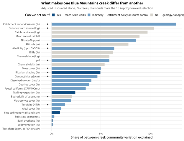
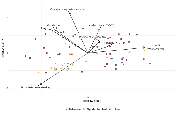
All 27 predictors together explain 46% of the compositional difference between creeks. Forward selection on adjusted R-squared, with each step permutation-tested, retains 10 of them and 42%.
| Rank | Driver | Can we act on it? | Alone | p | q | In final model |
|---|---|---|---|---|---|---|
| 1 | Catchment imperviousness (%) | Indirectly — catchment policy or source control | 13% | < 0.001 | 0.002 | 2.8% |
| 2 | Distance from source (log) | No — geology, topography, weather | 10% | < 0.001 | 0.002 | 4.5% |
| 3 | Catchment area (log) | No — geology, topography, weather | 9.7% | < 0.001 | 0.002 | — |
| 4 | Mean annual rainfall | No — geology, topography, weather | 8.9% | < 0.001 | 0.002 | — |
| 5 | Nitrate-N (ppm) | Indirectly — catchment policy or source control | 8.6% | < 0.001 | 0.002 | — |
| 6 | Altitude (m) | No — geology, topography, weather | 7.8% | < 0.001 | 0.002 | 2.6% |
| 7 | Alkalinity (ppm CaCO3) | Indirectly — catchment policy or source control | 6.4% | < 0.001 | 0.002 | 3.1% |
| 8 | Riffle (%) | No — geology, topography, weather | 6.2% | < 0.001 | 0.002 | — |
| 9 | Channel slope (log) | No — geology, topography, weather | 5.9% | < 0.001 | 0.002 | — |
| 10 | pH | Indirectly — catchment policy or source control | 5.9% | < 0.001 | 0.002 | 2.8% |
| 11 | Channel width (m) | No — geology, topography, weather | 5.4% | < 0.001 | 0.002 | — |
| 12 | Moss cover (%) | Indirectly — catchment policy or source control | 5.0% | < 0.001 | 0.002 | 2.7% |
| 13 | Riparian shading (%) | Yes — reach-scale works | 5.0% | < 0.001 | 0.002 | 1.2% |
| 14 | Conductivity (µS/cm) | Indirectly — catchment policy or source control | 4.7% | < 0.001 | 0.002 | 0.9% |
| 15 | Dissolved oxygen (mg/L) | Indirectly — catchment policy or source control | 4.0% | < 0.001 | 0.002 | — |
| 16 | Detritus cover (%) | Indirectly — catchment policy or source control | 3.8% | 0.002 | 0.003 | — |
| 17 | Faecal coliforms (CFU/100mL) | Indirectly — catchment policy or source control | 3.5% | 0.002 | 0.003 | — |
| 18 | Trailing vegetation (%) | Yes — reach-scale works | 2.4% | 0.008 | 0.012 | — |
| 19 | Bedrock (% of substrate) | No — geology, topography, weather | 2.0% | 0.011 | 0.016 | 2.0% |
| 20 | Macrophyte cover (%) | Indirectly — catchment policy or source control | 2.0% | 0.021 | 0.028 | — |
| 21 | Turbidity (NTU) | Indirectly — catchment policy or source control | 1.4% | 0.046 | 0.059 | 2.1% |
| 22 | Algal cover (%) | Indirectly — catchment policy or source control | 1.0% | 0.084 | 0.103 | — |
| 23 | Fine sediment (% silt and clay) | Yes — reach-scale works | 0.8% | 0.127 | 0.149 | — |
| 24 | Substrate coarseness | Indirectly — catchment policy or source control | 0.3% | 0.268 | 0.301 | — |
| 25 | Bank overhang (%) | Yes — reach-scale works | 0.1% | 0.377 | 0.392 | — |
| 26 | Sedimentation (%) | Yes — reach-scale works | 0.1% | 0.371 | 0.392 | — |
| 27 | Phosphate (ppm, as PO4 or as P) | Indirectly — catchment policy or source control | 0.0% | 0.668 | 0.668 | — |
9.5.1 What we can act on, and what we cannot
| Can we act on it? | Drivers | Strongest | Retained | Combined unique share |
|---|---|---|---|---|
| Yes — reach-scale works | 5 | Riparian shading (%) (5.0%) | 1 | 1.2% |
| Indirectly — catchment policy or source control | 14 | Catchment imperviousness (%) (13%) | 6 | 14% |
| No — geology, topography, weather | 8 | Distance from source (log) (10%) | 3 | 9.2% |
Four things follow for management.
Catchment imperviousness is the strongest single driver, and it is the one you have most control over — through planning controls, stormwater treatment and development consent, rather than through creek works. On its own it explains 13% of between-creek compositional difference (Table 9.9), and it is the first variable forward selection picks. Chapter 4’s caveat applies: imperviousness is part measured and part assumed — roof area is measured from Council’s building polygons, while the paving beside it and the sealed share of the road reserve are not — so the estimate is good enough to rank creeks and not good enough to set a threshold on. And read Section 9.4.3 before treating the reach-scale levers below as a substitute: most of what imperviousness explains is shared with chemistry and habitat rather than unique to it, which is consistent with it acting through them and equally consistent with all three tracking the same catchments.
Riparian shading is the strongest reach-scale lever (Table 9.10). It explains 5.0% on its own, survives forward selection with a unique contribution of 1.2%, and it is the one variable in this list that a revegetation program changes within a decade. Trailing vegetation, the next riparian variable down, ranks 18 of 27 on its own and does not survive selection. Read shading as a state: Section 9.3.2 shows the recorded rise in shading is recording rather than creeks, so a site that scores high is genuinely shaded, and a site whose score has gone up has not necessarily gained canopy.
Moss cover is a symptom rather than a lever. On its own it explains 5.0% of between-creek difference, ranking 12 of 27, and it does survive forward selection. But once the rest of the model is in place its unique contribution is 2.7% — 5 of the 10 variables retained, against 2.8% for imperviousness. So about 46% of what moss explains on its own the rest of the model already knew — riparian shading, substrate and the water chemistry — which is what you would expect of something that grows on stable, shaded, coarse substrate in clean water. It is a fair field-visible summary of the conditions sensitive invertebrates need, and it is quick to record, so keep recording it. Just do not read it as a driver, and do not plant moss.
Most of the ranking is geography. Distance from source, catchment area, altitude and rainfall between them account for the largest share, and none of them can be changed. A creek near the top of its catchment supports a different assemblage from one near the bottom, and that is not a management problem. The practical implication is that creeks must be compared with creeks like them. A rating system that does not condition on position in the network will penalise headwater sites for being headwater sites.
Sedimentation and phosphate, the two variables a reader would most expect to matter, do not. Site-mean sedimentation explains 0.1% (p = 0.371) and site-mean phosphate 0.0% (p = 0.668) of between-creek composition, and neither is retained by forward selection. Phosphate is worse than that: it ranks last of the 27 candidates, and it is the only one whose adjusted R-squared is negative (-0.36%, which means it predicts between-creek composition less well than a variable of pure noise would).
Chapter 6 gets to the same place by a different route. 54% of the phosphate readings in the database are below the laboratory detection limit, so an apparent association between phosphate and the health score is largely an association with how often the result cleared that limit — a statement about the laboratory test, not about the creeks. The result here points the same way from the opposite direction: there is no association to explain away in the first place. On this evidence phosphate is a candidate for neither a compositional nor a condition metric. Composition and condition are not the same response and the variables that rank them differ — but phosphate ranks neither.
9.6 What moves a creek between visits
The same-day site description gives a second, harder test. For 522 samples at 60 sites there is a habitat description, a water quality reading and a flow state recorded on the day the net went in. Partialling out creek identity, which takes 51% of the compositional inertia on this subset, leaves the question: what makes this visit to this creek different from the last one? (22 water quality sample codes carry more than one site description, 25 surplus rows in all; the first is used rather than the mean, because where two same-day descriptions of the same reach disagree their mean describes neither.)
The flow state block is the new one here. Flow is the obvious candidate for the thing that moves a creek between visits, and the natural assumption has always been that nobody was measuring it. In fact you have been, since 2008, in a free-text box on the site description sheet — Section 9.3.3 describes how it was recovered. The block below is the first test of it against composition.
vegan::RsquareAdj returns these as shares of total inertia even for a conditioned model, so each has been divided by 0.49 — the within-creek share of the ordination’s own inertia, read off its inertia components rather than off an adjusted R-squared — to express it as a share of the within-creek variation, which is what this section is about.
| Block | Block alone | Unique share |
|---|---|---|
| Visit habitat | 4.0% | 2.3% |
| Sampling effort | 2.6% | 2.2% |
| Climate | 1.9% | 1.1% |
| Time | 1.7% | 0.4% |
| Same-day water quality | 1.7% | 0.3% |
| Flow state | 1.0% | 0.2% |
| The six unique shares added up | 6.5% | |
| Held jointly, counted once | 2.5% | |
| All six together | 9.0% | |
| Left over | 91% |
Almost nothing you measure predicts how a creek’s community differs between one visit and the next, and that survives the arrival of flow state. Every measured variable together explains 9.0% of the compositional variation that remains once creek identity is accounted for, and the largest single variable is not an environmental one — the number of animals counted adds 2.2% that no other block already holds, nearly as much as the 10 same-day habitat variables together (2.3%), and it has more than twice the pseudo-F of any other term. Same-day water quality contributes 0.3%. Flow state, tested here for the first time, contributes 0.2% — the smallest of the six on both columns of the table.
Two things about Table 9.11 matter, because getting either wrong is how a reader ends up with a number that means something other than what they think. The first is that the six unique shares add to 6.5% while the six blocks together take 9.0%. The 2.5% difference is not a rounding error: it is the part the blocks hold jointly. Rainfall, riffle proportion and flow state are all partly saying the same thing about how much water is in the channel, so that part belongs to all three and to none of them, and it cannot be handed to any single row. The second is that the two columns answer different questions and need not rank the blocks the same way — a block that overlaps others heavily can track a lot and add almost nothing. Every superlative in this section is computed from the table rather than typed: a superlative in prose is exactly the claim that quietly stops being true the next time a model is refitted.
Everything above is a share of what is left within creeks, which is itself only 49% of the total — creek identity takes the rest. So 91% of the within-creek variation is untouched by anything on the list.
| Term | Pseudo-F | p | q |
|---|---|---|---|
| Sampling effort (log animals counted) | 10.1 | < 0.001 | 0.010 |
| 12-month drought index (SPI-12) | 4.3 | < 0.001 | 0.010 |
| Riparian shading (%), on the day | 2.8 | 0.002 | 0.010 |
| Time (decades) | 2.7 | 0.002 | 0.010 |
| Riffle (%), on the day | 2.5 | 0.014 | 0.035 |
| Moss cover (%), on the day | 2.3 | 0.009 | 0.026 |
| Macrophyte cover (%), on the day | 2.1 | 0.009 | 0.026 |
| Trailing vegetation (%), on the day | 2.1 | 0.008 | 0.026 |
| Rainfall, previous 90 days | 2.1 | 0.018 | 0.040 |
| Dissolved oxygen (mg/L), on the day | 1.8 | 0.032 | 0.060 |
This design is not underpowered, and a negative result used to close off a line of investigation has to say so. The conditioned ordination leaves 60 units of within-creek inertia and a residual of 52 on 438 degrees of freedom. Each term’s critical value is read straight off its own permutation distribution — the 95th percentile of the 999 permuted F statistics vegan already stores for it — so the bar ranges from 0.3% of within-creek compositional variation for the easiest term to 0.4% for the hardest. Taking the hardest, because the claim is about any single variable, the marginal test would have separated anything explaining more than about 0.4% from the permutation null at the 5% level, and 10 of the 20 terms tested do clear that bar.
Two instruments, and the sentence has to survive both. The figure above is the null this test actually uses. Referring the same statistic to an F distribution instead — the 95th percentile of an F on 1 and 438 degrees of freedom — puts the bar at 0.8%, about twice as high, because a marginal term in a partial ordination on a Bray–Curtis distance is not F-distributed and its permutation null is the tighter of the two. Both numbers are given because the sentence they support closes off a line of investigation, and a bound that depends on an undeclared choice of reference distribution is not a bound. What the section rules out is a large visit-level driver, not a small one: the ceiling on anything you measure but that has not turned up here is under one per cent on either instrument — about 0.4% against the permutation null and 0.8% against the parametric one.
That cuts two ways. It means a single visit’s water chemistry tells you almost nothing about the animals you will find that morning, which agrees with chapter 6’s finding that three-year site means predict the health score far better than spot readings. It also means that the large unexplained fraction in Section 9.4 is not a failure to measure the right things at the reach scale — it is the irreducible stochasticity of netting invertebrates.
9.6.1 Flow state: measured at last, and small
Flow state’s 0.2% needs care, because it is easy to get a much larger number by accident and the larger number would be wrong.
Flow state is recorded on 921 of the 1,502 edge stream samples — nearly twice the 522 that carry every block in the partition. Tested on all of them as a six-level factor, with the permutations restricted within creek, it looks substantial: 2.2% of total compositional variation (pseudo-F 4.19, p = 0.001), larger than any unique share in Table 9.11. That comparison is invalid. Restricting permutations within creek makes the test honest — it stops the p-value being inflated by creek differences — but it does nothing to the estimate. Creeks differ systematically in how much water runs down them, so an unconditioned R-squared for flow state is substantially a restatement of which creek the sample came from, which is the thing this section partials out.
Conditioning on site, rather than merely blocking the permutations, more than halves it — but the two figures have to be put on one base before they can be compared at all. That 2.2% is a share of total inertia; the same constrained inertia is 4.4% of within-creek inertia, which is the base the conditioned figure uses. Against that, flow state holds 1.7% of within-creek variation on the same 921 samples (pseudo-F 2.94, 5 df, p = 0.001; on the linear scale rather than as a factor, 1.1%, p = 0.001) — a drop of 2.7 points, not the 0.5 that subtracting the two published shares from one another would suggest. That is a real effect, significant on any reading, and it is the number to quote for how much flow state moves a creek’s community.
It is still small — on the partition set it is the smallest of the six on both columns of the table. Three different numbers describe how small, and mixing them up is the easiest mistake to make in this section, so here they are side by side.
| Question | Samples | Share |
|---|---|---|
| How much does flow state move a creek’s community? | 921 | 1.7% |
| How much does it track on the full-block subset, alone? | 522 | 1.0% |
| How much does it add that no other block already has? | 522 | 0.2% |
The first row of Table 9.13 is the one to quote when someone asks what flow state does. The third is the one that belongs in the partition. Most of what flow state knows, the visit habitat description and the climate terms already knew: riffle proportion, moss cover, bank overhang and 90-day rainfall are all partly descriptions of how much water is in the channel. In the single conditioned ordination behind Table 9.12, flow state ranks 16 of the 20 terms and does not reach significance (pseudo-F 1.1, 5 df, p = 0.205). Both statements are true: flow state is significant when it is the only thing asked about on every sample that carries it, and it is not significant once the other 19 terms are asked about alongside it on the smaller subset that carries all of them.
The variable everyone nominated as the likely missing driver has now been measured, and it is not the missing driver. That makes Section 9.6’s conclusion stronger rather than weaker. It is no longer “the thing that would explain it has not been recorded”; it is “the thing that would explain it has been recorded on 921 visits, it moves the community significantly, and it moves it by 1.7%.”
Two qualifications. The first is that this is an ordinal judgement by a field officer, not a discharge measurement: six levels, no calibration between officers, no information about the days before the visit. A gauged hydrograph would test antecedent flow, time since the last flushing flow, and whether the sample sat on a rising or falling limb — none of which a single word on a field sheet can carry, and all three are what dq:stream-gauges above asks for.
The second is that flow state does something much larger elsewhere in the report. It is the strongest visit-level predictor of dissolved oxygen (Section 6.7), where one step up the scale adds 2.70 percentage points of saturation (95% CI 1.95 to 3.45) or, on the other scale the same probe reports, 0.33 mg/L (0.25 to 0.40), on 870 and 879 samples respectively — one effect written twice, not two findings. Meanwhile it moves none of the four metrics the health rating is built from, and moves the published score by +0.001 points per step (p = 0.96, chapter 13).
9.7 What would make this chapter wrong
Five things, in the order in which they would matter.
Association, not causation, and no intervention anywhere in it. Creeks with a lot of shading differ from creeks with little in many ways besides shading. Nothing here shows that revegetating a degraded reach would change its community — only that shaded creeks hold different communities from unshaded ones. The ranking says where an intervention is plausible, not where it is proven. Chapter 17 is where the design for proving it lives.
The block ranked first is the block measured worst. Section 9.3.2 says what that costs and Section 3.6.2 diagnoses it; the ranking survives year-detrending and survives restricting to the described period, so it stands. But a block ranked first on percentages estimated by eye is not measured as cleanly as one ranked below it on instrument readings, and the worst-affected variables — algal cover, macrophyte cover, detritus cover — should be read as indicative. A rise in a recorded habitat variable is not evidence of a change in the creek.
The habitat and water quality blocks are site-level, so their unique fractions are between-creek fractions. They are not competing on equal terms with time and climate, which vary within a creek. That is why Section 9.5 exists, and the between-site ranking is the result to quote. It is also why a falling unique fraction proves nothing on its own: with 1,230 samples spread over 73 creeks, adding 13 site-level columns of pure noise cuts imperviousness’s unique share from 3.6% to 2.9% without meaning anything at all (Section 9.4.3).
And the same arithmetic inflates the blocks’ own unique shares, which is the more consequential half. Section 9.4.1 runs the control against each block instead of against one variable: 13 columns of site-level noise earn 4.3% where the real habitat block earns 7.9%, and the baseline rises with the width of the block, so a wide block and a narrow one are not comparable on unique share at all. What that costs is the effect sizes, and only the effect sizes. The ordering is unaffected — habitat leads on the published shares and net of noise alike — but no percentage in Table 9.5 should be repeated outside this chapter without its baseline, the “order of magnitude more than imperviousness” comparison is withdrawn, and the recommendation the partition supports (R10, a riparian and geomorphic panel) is entitled to the ordering and not to the size of the gap. The fix is one target, not a redesign, and Section 9.4.1 names it.
18% of samples are absent from the full-block model, because they sit at sites with no delineated catchment, no site description, or too few water quality readings. The 73 sites that remain are the modern network; the historic
K*,L*andM*sites are largely gone. The partition describes the network as it is now.Edge habitat only, family level only, streams only — chapter 8’s three restrictions, for chapter 8’s three reasons: riffle sampling stopped after 2007, order-level records confound taxonomic resolution with composition, and wetland assemblages are different assemblages rather than degraded stream ones. The two laboratory discontinuities the era corrections handle were found in the data rather than documented (Section 3.7.6), so those corrections inherit that uncertainty: a parameter that genuinely changed at the same time as the reagent cannot be separated from the reagent.
One thing this chapter does not support, though the reverse would be a natural reading of it: do not add a water quality component to the rating on compositional grounds. The water quality block uniquely explains 3.8% of composition, less than half what physical habitat explains, and the highest-ranked single parameter between creeks is Nitrate-N (ppm), 5 of 27, behind only Catchment imperviousness (%), Distance from source (log), Catchment area (log), and Mean annual rainfall. Chapter 6’s case for reporting water quality — that it is diagnostic of what is wrong — stands on its own; the case that it separates sites better than the animals already do does not.
| Item | Value |
|---|---|
| Data layer built | 2026-08-30 12:56 |
| R version | R version 4.4.3 (2025-02-28) |
| Full-block analysis set | 1,230 samples, 73 sites, six blocks |
| Between-creek set | 74 sites on 63 waterways, 27 candidate drivers |
| Within-creek set | 522 samples, 60 sites with same-day habitat and water quality |
| Flow-state set | 921 samples carrying a normalised flow state |
| Model fits | read from the targets graph in R/_targets.R |