| Population | n | Where it comes from | Who uses it |
|---|---|---|---|
| Named in methods Appendix 2 | 12 | The methods document: four lower-altitude and eight higher-altitude creeks | The methods document. Nothing in the data layer counts only these twelve |
| Flagged reference in the site register | 17 | Sites.Classification in the macroinvertebrate database, carried into the data layer as disturbance_tier. Appendix 2’s twelve plus 5 historic sites |
Anything counting reference sites, including the chemistry yardstick below |
| With a rated edge stream sample | 16 | 212 samples, 1998–2024; excludes the one reference wetland, which is scored on a different band table | Anything pooling reference samples |
| With a rated edge stream sample from 2010 on | 11 | 145 samples | Chapter 13’s discrimination test, which is the number Part III leans on |
| With a delineated catchment | 15 | Chapter 4’s delineation | Anything conditioning on catchment area, imperviousness or fire |
12 An external check on the reference set
Blue Mountains City Council Healthy Waterways — statistical analysis
12.1 What this chapter is for
Part III asks whether your waterway health rating works. Every test in it is measured against the same thing: your reference sites. The bands are percentiles of what those creeks produced, so calling a sample Excellent is a statement that it looks like the top of the reference set. Chapter 13’s discrimination test, chapter 14’s band reset and chapter 15’s revision all inherit that, and none of them can be more trustworthy than the benchmark underneath.
So the first question in Part III is not whether the rating works. It is whether the benchmark is the right benchmark — and that is a question your own data cannot answer, because the tiers and the bands are both yours. You need something from outside.
There is exactly one thing from outside. The NSW Department of Climate Change, Energy, the Environment and Water has run AUSRIVAS-protocol macroinvertebrate sampling across the state since the mid-1990s — Turak et al. (1999) report sampling 250 reference sites statewide in autumn and spring 1995, and no program document giving an exact start date was available for this report — its public release covers this study area, and in one case it sampled the same creek within a hundred metres of one of your sites. This chapter is what that archive can and cannot tell you.
The short version, and the rest of the chapter is the working:
- It corroborates, at one site. Two archive sites 93 m and 515 m from your reference site
75BKTRon Reedy Creek returned the same verdict — band B, significantly impaired — on all 4 model runs they produced, 13 years apart, and your own scores at that site say the same thing. It is the only one of your 17 reference sites an outside program has ever assessed — the archive reaches 8 sites in your network in all (Figure 12.1), but this is the only one of them Council calls reference — and the two assessments agree. - It cannot be pooled. 7 of the 8 archive sites in good enough condition to be reference candidates are on the wrong kind of creek entirely, and 3 of the 4 rating factors cannot be computed from an archive sample and mean the same thing. So the archive tests your reference set. It does not extend it.
- Two sites is a spot check, not a validation. One reference site out of 11 in the 2010-onward analysis set has any external evidence at all, and all of it predates the 2019–20 fires. What it would take to do better is costed at the end of the chapter, and it is one field season.
12.2 The data behind this chapter
Each question and request below is set out again in What we need from you, with what it blocks, what an answer is worth and what it would cost you to find, ranked against every other ask in the report.
12.2.1 What this chapter uses, and where it came from
Provenance — the NSW AUSRIVAS archive, held by DCCEEW, extracted August 2026.
105 sites in the buffered study window, sampled 1994–2018, of which 12 lie within 2 km of one of your monitoring sites. Family-level counts, field and laboratory chemistry, and a stored AUSRIVAS observed-to-expected score with a published band. Extracted to R/data/external/ausrivas/ and loaded by data-layer/external/13-ausrivas-nsw.R; the comparison tables the chapters quote are built once in 21-ausrivas-comparison.R and cached to data/derived/ausrivas_comparison.rds. This is the only external macroinvertebrate data in the report, and chapter 7’s phosphate non-detect evidence comes from the same archive. That phosphate comparison is species-sensitive and neither program’s records settle it: nothing says whether our readings are phosphate as PO4 or as P, the two differ by a factor of three, and the direction of chapter 7’s argument turns on the answer (dq:phosphate-units).
Value: high. Costs you: minutes. Refer to it as
dq:ausrivas-provenance.
12.2.2 What is wrong with it
Problem — the archive’s stored O/E scores stop on 23 June 2011, so the external check says nothing about the 13 years of Council’s own record that follow it.
The archive’s site register runs to 2018 and its other analytes with it, but the AUSRIVAS model scores stop in 2011. That matters more than it looks: every external observation in chapter 12 predates the 2019–20 fires, which chapter 14 shows lowered the reference benchmark by about half a rating point at the catchments that burnt. Reedy Creek’s catchment burnt entirely. So the external evidence describes a reference set that no longer exists in that state.
Blocks: Any claim that the reference set is externally corroborated as it stands today. Value: high. Costs you: minutes. Refer to it as
dq:ausrivas-indices-stop-2011.
Problem — the extraction window is the buffered DEM extent, so it catches the whole South Creek program in western Sydney.
105 sites in the window; 12 within 2 km of one of yours. Any statistic over all 105 is a statement about western Sydney, and the difference is not small — the far sites include nutrient-enriched lowland creeks downstream of a sewage treatment plant. Everything in chapter 12 is computed on the 12, and the distances were recomputed from coordinates rather than taken from the archive’s own site table.
Blocks: Any window-wide statistic quoted as if it described the Blue Mountains. Value: high. Costs you: minutes. Refer to it as
dq:ausrivas-window-not-bmcc.
Problem — “reference site” resolves to 11, 12, 15, 16 or 17 sites depending on which definition is in play.
Methods Appendix 2 names twelve. The site register flags seventeen (sixteen Reference plus one ReferenceWetland), the extra five being historic sites the methods document does not name. Sixteen carry a rated edge stream sample, eleven carry one from 2010 on, and fifteen have a delineated catchment. All five are defensible; the defect is quoting one and meaning another. Chapter 12’s opening table (Table 12.1) pins them down and the rest of Part III points at it.
Blocks: Any count of reference sites, and any band derivation that says which creeks it pooled. Value: high. Costs you: minutes. Refer to it as
dq:reference-set-five-counts.
12.2.3 Questions only you can answer
When were the reference and ‘slightly disturbed’ tiers last looked at, and is there a record of who set them and on what evidence?
The tiers are a lookup, not a measurement, and two cases in chapter 12 show them coming apart from the data. 75BKTR (Reedy Creek) is tiered reference and both an external national model and your own scores put it below reference condition. 11BMG (Megalong Creek at Narrow Neck) is tiered urban, and an external model scored the reach beside it band A on 18 of 23 runs while your own 17 samples there average 4.24 — its catchment is 1.2% impervious, inside the range of your reference catchments. Neither is necessarily wrong, because a tier is a judgement about the catchment. But if there is a review cycle we should know its date, and if there is not, that is worth saying in the report.
Refer to it as
dq:reference-tier-review.
(DCCEEW, not you) Which unit was TKN actually reported in? The per-row Units field and the t_WaterQualityTypes lookup both say µg/L, but the stored values are only sensible as mg/L. And is -999 in O/E50 and band a null?
A thousandfold error waiting to happen, in a dataset the report leans on as its only external yardstick. Cheap to confirm and expensive to get wrong.
Refer to it as
dq:ausrivas-units.
K40, K43, K53, P7 and W14 are classified Reference in the database but are not in methods Appendix 2 — were they ever reference sites, or is that classification inherited from something else?
They hold 33 macroinvertebrate samples between them, and they are in every count that reads the database classification and in none that reads the methods document. That is why “the reference set” is seventeen sites in some places in this report and twelve in others. Either answer is fine — we just need to know which. Four of the five already have a working position recovered from their stored easting/northing (K43 and K53 confirmed, K40 and W14 probable) and a delineated catchment; only P7 has neither, so P7 is the only one whose location we still need.
Refer to it as
dq:reference-historic-five.
12.2.4 What would answer them
Would you be willing to run one season’s macroinvertebrate sampling to the AUSRIVAS protocol alongside your own, at the reference sites — and could DCCEEW be asked to sample the same reaches in the same season?
The whole archive holds exactly one visit pair that is genuinely comparable to one of yours: same habitat, same austral season, twelve days apart. One co-located field round at the twelve archive sites in the proximity set would produce twelve same-day pairs — more than the archive has accumulated in thirty years — and run at the eleven reference sites instead it would give the first external assessment of ten of them. The protocols are already compatible: both sample edge and riffle, both identify to family, both use the same SIGNAL grade tables, and they pick to a similar effort (median edge richness 15 against 14). Nothing needs to be developed first. This is the single most concrete data request in the report.
Refer to it as
dq:ausrivas-colocated-round.
(DCCEEW) Is t_AUSRIVASPhysChem available anywhere? It is empty statewide in the public extract.
Only needed if we want to re-run the AUSRIVAS models rather than accept the published O/E50 scores, which is not currently the plan. Low priority, on the list so it is not rediscovered later.
Refer to it as
dq:ausrivas-physchem.
12.3 Which sites are “reference”, and how many
Before any of that: reference does not name the same set of creeks in every part of this book, and the counts differ enough to matter. This chapter enumerates five defensible answers, and those five run from 11 to 17. That is this chapter’s range, not the book’s: two narrower populations exist downstream and both sit below the floor — chapter 14’s percentile-calibration set and chapter 15’s holdout, each of which drops reference creeks again to keep its test honest, and each of which states its own count where it is used. Neither is a count of the network.
The gap between Appendix 2’s twelve and the register’s 17 is 5 historic sites — K40, K43, K53, P7, and W14 — which carry a Reference classification in the database and hold 33 macroinvertebrate samples between them. All 5 have a surveyed easting and northing, and 4 of them have a delineated catchment; P7 has no derived latitude and longitude and no catchment, and neither does the Appendix 2 site 27GLNR — those two are the whole of the gap between the register’s 17 and the 15 in Table 12.1. They are in every count that reads disturbance_tier and in none that reads the methods document. The gap between 11 and 17 is those five plus the single reference wetland, 28EHZR, which is scored on a different band table and is chapter 11’s problem, not Part III’s. The five do have rated edge stream samples, so they sit inside the 16; the wetland is the only site in the register with none, and it is the whole of the gap between 16 and 17.
Where this chapter says “reference site” without qualification it means the 17 in the register, because that is the population the chemistry yardstick below is computed over. Where a number needs one of the other four it says so.
12.4 The archive, and what is in it
The NSW AUSRIVAS archive is a different organisation running a nationally standardised index over the same country. It is the only external macroinvertebrate data this report uses, and chapter 7 leans on its water quality half as well (Section 7.5.1), so this section owns its provenance.
What it is: 105 sites in the extraction window, sampled between October 1994 and May 2018, extracted to R/data/external/ausrivas/ and loaded by data-layer/external/13-ausrivas-nsw.R. It carries family-level macroinvertebrate counts, field and laboratory water chemistry, and — the part that matters here — a predictive model score. AUSRIVAS compares the families actually found against the families a model predicts for a site of that type, in that season and habitat, and reports the ratio as O/E50 with a band from X (richer than predicted) through A (reference equivalent) to D. Appendix A records the extraction; the data section above records what we had to guess.
Three limits, before any number is read.
The window is not the Blue Mountains. The extraction window is the buffered DEM extent, not the local government area, and it catches the whole South Creek program in western Sydney. Of the 105 sites, 12 lie within 2 km of one of your monitoring sites. Any statistic computed over all 105 is a statement about western Sydney. Everything below is computed on the 12 unless it says otherwise — the search for reference candidates deliberately reaches into the whole window, and says so — and the distances were recomputed from the coordinates rather than taken from the archive’s own site table.
The archive sets the window, not you. The stored AUSRIVAS indices stop on 23 June 2011, while your macroinvertebrate record runs to 20 August 2024. Nothing in this chapter is a statement about the 13 years of your own record that follow that date — measured against today it is 15 years, which is the figure Section 12.8 prices the fieldwork against — and in particular nothing in it is a statement about the reference set after the 2019–20 fires, which chapter 14 shows lowered the benchmark at the catchments that burnt (Section 14.4.1).
The models cannot be re-run. The physical-chemical table the AUSRIVAS models need is empty statewide in the public extract, so only the stored observed-to-expected ratio is usable, exactly as published. That is a want on the data list above, addressed to DCCEEW rather than to you, and it is a low priority — accepting the published score is the plan.
12.5 What the archive says about Reedy Creek
Start with the one place where an outside program and yours sampled the same reference creek.
| Archive site | Name | Council site | Separation (m) | Visits | Model runs | O/E range | Bands | Period |
|---|---|---|---|---|---|---|---|---|
| 22136 | Reedy Ck @ Kedumba Valley Rd | 75BKTR | 93 | 1 | 2 | 0.80–0.81 | 0 A, 2 B | May 2011 to May 2011 |
| HAWK106 | Reedy Ck d/s Spring Ck | 75BKTR | 515 | 2 | 2 | 0.63–0.77 | 0 A, 2 B | Apr 1998 to Nov 1998 |
2 archive sites sit within 515 m of 75BKTR, Reedy Creek — one of your reference sites in the Warragamba Special Area, and one of the 11 reference sites carrying the 2010-onward samples the rest of Part III rests on. Between them, in Table 12.2, they produced 4 model runs across 3 visits, in 1998 and 2011, and every one of them came back band B, with O/E between 0.63 and 0.81.
The two programs agree on the water, which is how we know this is the same reach and not a mismatch of location: the archive’s median field conductivity is 93 µS/cm at the closer site and 58 at the further one, against a median of 83 µS/cm across your own 3 readings at 75BKTR.
And your own scores say the same thing. The 6 rated edge samples at 75BKTR, from 3 visits between 2017 and 2019, rate 3 Fair, 2 Good, 1 Poor, averaging 2.48 on the five-point scale — which is Fair.
Two independent assessment systems, built by different organisations on different principles, agree that one of your reference creeks is not in reference condition. That agreement is the strongest external result in this report.
12.5.1 What that does and does not establish
The result is easy to inflate in either direction, so be exact about what it is.
It is not a defect in either system, and it is not a mistake. Reedy Creek is a catchment in a protected water supply special area, its 1,870 ha upstream area is 0.3% impervious, and your tier records that honestly. But the tier is an attribute of the catchment, while the reference bands are percentiles of the assemblages found there. Where the two come apart, the bands inherit the gap. This is the constraint Section 14.3 describes in the abstract, arriving as a specific creek — and it is why chapter 15’s revised rating drops 75BKTR a class (Section 15.4.2) rather than that being a bug in the revision.
It is a spot check on one site, not a validation of the reference set. One of the 11 reference sites in the 2010-onward analysis set has external evidence. The other 10 have none, and nothing here licenses a claim about them. Two archive sites near one of your sites is what the archive happens to hold, not a designed test.
The two records do not overlap in time. The archive assessed Reedy Creek in 1998 and 2011; your own samples there run 2017–2019. They agree, but they are not two measurements of the same water on the same day, and neither is recent: 75BKTR’s catchment burnt 100% in the 2019–20 fires, after the last observation in this chapter. Nothing here describes the reference set as it stands now.
A third archive site is assigned to 75BKTR and disagrees, and it is reported rather than dropped. 22103, Kedumba River @ Murphy’s Crossing, sits 1,573 m away and returned 1 A and 1 X over 2 runs. It is on the Kedumba River, not Reedy Creek, which is why it is not in Table 12.2 — at that separation, proximity is a proximity of points and not of reaches.
12.5.2 The proximity set as a whole
Reedy Creek is not unusual within the local set. Figure 12.1 puts every archive model run at the 12 sites within 2 km beside your nearest site.
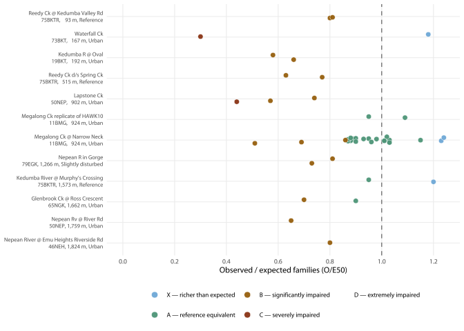
32 of the 44 model runs at these 12 sites fall below the model’s expectation, and 18 are called impaired — the bands allow for ordinary variation around 1.0, so the second number is the smaller. Read that as description and not as a rate: the runs are nowhere near independent. 23 of the 44 come from a single site, and every visit contributes an edge and a riffle run scored by different models. Only the 1.0 line is drawn, because it is the one threshold the four seasonal and habitat models share: the A/B boundary is model-specific, running from 0.82 to 0.89 across the four.
12.6 The reference set cannot be extended, only tested
The obvious hope is that a nationally run program could add sites to the reference set and relieve the constraint that limits the whole of Part III. It cannot, for two independent reasons, and both are set out in full because the temptation to pool is real.
12.6.1 Most of the good-condition sites are the wrong kind of creek
Taking every archive site with at least three model runs and a mean observed-to-expected ratio at or above 0.85 gives 8 candidates. 7 of them are 12–22 km away, on the Werriberri (Monkey) Creek, Jenolan River, Coxs River, and Jocks Creek, and their water says what they are: median field conductivity 70–510 µS/cm and median alkalinity 16–110 mg/L, against 54 µS/cm (n = 140 readings) and 6 mg/L (n = 135) across your 17 reference sites. These are limestone-country streams west of the escarpment, not soft sandstone headwaters. A site scoring well on a limestone river is in good condition for a limestone river — that is exactly what a predictive model is for, and exactly why its score cannot be transplanted.
One candidate survives the stream-type test, and it is more interesting than it looks. HAWK10, Megalong Ck @ Narrow Neck, sits 924 m from your 11BMG, with median conductivity 47 µS/cm and alkalinity 10 mg/L — squarely inside your reference range — and the archive scored it band A on 18 of 23 runs between 1994 and 2009. Your own record agrees: 11BMG has 17 rated edge samples from 2006–2024 averaging 4.24 (13 Excellent, 4 Good), and its catchment is 1.2% impervious against a median of 0.0% and a maximum of 1.9% across your 15 delineated reference catchments.
11BMG is tiered urban. An external model and your own scores both put it in reference condition, and the tier lookup does not. That is not an argument for repointing it tonight — the tier is a catchment judgement and 924 m is not nothing — but it is a concrete example of the reference set being defined by a lookup rather than by the data, and it is the kind of case a periodic review of the tiers would catch, and it is on the data list above (dq:reference-tier-review).
12.6.2 Three of the four rating factors are not exchangeable
Your rating averages four factors, and pooling a foreign sample into the reference set means computing all four from it and having them mean the same thing.
| Factor | AUSRIVAS equivalent | Pool? | Reason |
|---|---|---|---|
| SIGNAL-SF | SIGNAL_SydneyFamilies | YES | Same grade table and same formula. Of the 95 families graded by both programmes, 95 carry an identical grade and 0 differ — both derive from the same published Chessman tables. Council’s rule reproduces AUSRIVAS’s stored value exactly on 100% of the samples it can be checked against. |
| n_families | TaxaRichnessFamily | NO | Council’s n_families is not a richness count. It reproduces an Access rule that counts DISTINCT (family, count) PAIRS, so a family recorded twice with different counts is counted twice. It is kept because every historical rating depends on it (03-metrics.R). AUSRIVAS’s TaxaRichnessFamily is a true distinct family count. The two are different quantities and the difference is not a constant, so no offset converts one into the other. |
| n_ept_families | EPTRichness | NO | The EPT family lists differ. Council’s list and the taxonomy-based list disagree on 14 families (ept_definition_comparison in the data layer), and AUSRIVAS’s EPTRichness follows the taxonomic definition. Reconcilable in principle by recomputing from raw counts, but not as stored. |
| pct_ept | not published | NO | Depends on total abundance, which depends on the subsample size each programme picks to. AUSRIVAS does not publish pct_ept, so it would have to be recomputed from counts taken under a different picking protocol. |
| the rating itself | AUSRIVAS band | NO | Different constructions, not different calibrations of one thing. Council scores each factor against percentile bands from its own reference sites; AUSRIVAS scores observed families against a MODELLED expectation for that site, season and habitat. A band is not a rescaled rating and the two need not agree even when the underlying metrics do. |
The one of the four in Table 12.3 that is exchangeable is exchangeable completely, which is unusual enough to record. Both programs grade families from the same published SIGNAL tables: of the 95 families graded by both, all 95 carry an identical Sydney-families grade and 0 differ, and your averaging rule reproduces the archive’s own stored SIGNAL-SF exactly on all 225 samples where a one-to-one check is possible. The two programs also pick to a similar effort: median edge-habitat family richness is 15 across 257 archive samples against 14 across 1,712 of yours.
The other three fail for documented reasons rather than suspected ones. Your n_families reproduces an Access rule that counts distinct family-and-count pairs, so it is not a richness count at all and no offset converts it into one — chapter 1 sets out the rule and what it does to the number (Section 1.2), and it is why n_families_strict exists. The EPT family lists differ. And pct_ept depends on the subsample size each program picks to, and is not published by the archive at all.
So the archive corroborates the reference set at one site. It does not extend it, and nothing in this report pools the two. An external program scoring a nearby undisturbed catchment is worth writing down even when its numbers cannot enter the same model — but a reference set is the one thing in this system that must not be quietly contaminated, and one exchangeable factor of four does not justify it.
12.7 Does the rating agree with a standardised index?
The direct test is to find visits where both programs sampled the same water at the same time and compare the two verdicts. Seasonality in macroinvertebrate assemblages is strong enough that a spring sample against an autumn one is not a comparison, so both the gap in days and the austral season of each visit are carried.
| Archive site | Council site | Sep. (m) | Habitat | Gap (d) | Season | O/E | Band | Council rating | SIGNAL-SF | EPT |
|---|---|---|---|---|---|---|---|---|---|---|
| 24007 | 19BKT | 192 | Edge | 12 | Autumn | 0.62 | B | Fair | 6.81 / 6.70 | 4 / 3 |
| HAWK10 | 11BMG | 924 | Edge | 61 | Autumn vs Summer | 0.69 | B | Good | 6.89 / 6.13 | 8 / 7 |
| HAWK10 | 11BMG | 924 | Riffle | 61 | Autumn vs Summer | 0.86 | B | Excellent | 6.94 / 6.74 | 10 / 11 |
| HAWK10 | 11BMG | 924 | Edge | 139 | Spring vs Summer | 0.87 | A | Good | 7.10 / 6.13 | 6 / 7 |
| HAWK10 | 11BMG | 924 | Riffle | 139 | Spring vs Summer | 1.15 | A | Excellent | 7.00 / 6.74 | 10 / 11 |
| 21097 | 46NEH | 1824 | Edge | 155 | Autumn vs Summer | 0.80 | B | Fair | 5.00 / 6.33 | 4 / 4 |
There is exactly 1 genuinely comparable pair. At 19BKT on 18 April 2007, you sampled the edge habitat 12 days before the archive sampled the same habitat 192 m away, both in Autumn. Every other pair crosses a season boundary, and two of them pair the same Council sample with two different archive visits that scored differently — band B and A — which is a useful reminder of how much of an assemblage score is the month it was taken in. Two rows are riffle samples, and your published bands do not apply to riffle — chapter 3 item 3 has the size of that bias — so their Council ratings are shown because they are what the system produces, not because they are defensible.
1 pair supports no model, and none is fitted. What Table 12.4 shows, read as description rather than inference, is a pattern worth naming:
The two programs largely agree on the animals and disagree on the verdict. Across the 5 pairs that are genuinely co-located — within 924 m — the underlying metrics track each other: SIGNAL-SF differs by less than a point on a scale running to 10, and EPT family richness by less than two families. The published words do not. 3 of those 5 archive assessments return band B, while the 3 Council samples they pair with are rated Fair, Good, and Excellent. (Over all 6 pairs in Table 12.4 it is 4 of 6; the extra pair is the distant one, below.) The one pair further off is also the one where the metrics themselves diverge, and it is instructive: at 1,824 m it pairs a Nepean River site with a Council site on Strathdon Creek. Proximity here is a proximity of points, not of reaches, and 2 km can cross a confluence.
That is what should be expected, and it is not a failure of either system. The two are different constructions, not two calibrations of one thing: you score each factor against percentile bands drawn from your own reference sites, while AUSRIVAS scores the families observed against a model’s prediction for that site, season and habitat. A band is not a rescaled rating. The agreement on SIGNAL-SF and EPT richness is the meaningful result — it says the two field and laboratory protocols are collecting the same information, which is the precondition for any future comparison.
12.8 What a co-located sampling round would buy
The honest summary is that the external check is real but thin: one comparable visit pair, 4 model runs at one reference site, and an archive whose indices stopped 15 years before this report was compiled — 13 years before the end of your own record. That thinness is itself the finding, and it prices a piece of fieldwork precisely.
- The protocols are already compatible where it matters. Both sample edge and riffle habitats, both identify to family, both use the same SIGNAL grade tables, and they pick to a similar effort. No methodological work is needed first.
- What is missing is contemporaneous data, not comparability. The two programs overlapped on the ground for 20 years — 1998 to 2018 — and produced 1 visit pair that can be compared, because neither program was ever asked to sample near the other in the same season.
- A single round would change that. Running the AUSRIVAS protocol alongside your own at the 12 sites in the proximity set, in one season, would give a same-day paired comparison at every one of them — 12 comparable pairs from one field round, against the 1 the whole archive holds. Better still, run it at the 11 reference sites instead: that is the population Part III actually depends on, and 10 of them currently have no external evidence at all.
Section 16.1’s seventh test asks whether a rating agrees with your own ecologists. This is the same idea pointed at an outside program instead, and it is the cheapest way to put a second external number against a rating system that currently has one.
12.9 What we can and cannot say
| Question | Answer | Confidence |
|---|---|---|
| Is there any external evidence on the reference set? | Yes, at one site. 2 archive sites 93 m and 515 m from 75BKTR returned band B on all 4 model runs they produced, across 3 visits in 1998 and 2011. | High for the site. The two programs agree on the water (93 and 58 against 83 µS/cm) so this is the same reach. |
| Does your own data agree? | Yes. The 6 rated edge samples at 75BKTR (2017–2019) average 2.48 — Fair. | High that the two verdicts agree; low that they describe the same period. The archive’s assessments are 6 to 21 years older than your own samples. |
| Does that validate the reference set? | No. 10 of the 11 reference sites in the 2010-onward analysis set have no external evidence at all, and every observation in this chapter predates the 2019–20 fires. | High. This is a spot check on one site, and it is not a designed test. |
| Can the archive add sites to the reference set? | No, on two independent grounds: 7 of the 8 candidates are limestone-country streams 12–22 km away, and 3 of the 4 rating factors cannot be computed from an archive sample and mean the same thing. | High for both. The exchangeability failures are documented mechanisms, not suspicions; the chemistry contrast is 70–510 µS/cm against 54. |
| Does the rating agree with a standardised index? | The metrics do; the verdicts do not. Across the 5 co-located pairs SIGNAL-SF differs by less than a point and EPT richness by less than two families. | Low as a test — there is 1 genuinely comparable pair in the whole archive, and no model is fitted. Moderate that the two protocols collect the same information, which is the part that matters for any future round. |
| How many reference sites are there? | Between 11 and 17, depending on what you are counting: 12 named in methods Appendix 2, 17 flagged in the site register, 16 with a rated edge stream sample, 11 with one from 2010 on, 15 with a delineated catchment. | High, and none of the five is wrong. The defect is quoting one and meaning another. |