| Current factor | Revised factor | Why |
|---|---|---|
| SIGNAL-SF (mean grade of families present) | Percentage of individuals in tolerant families (SIGNAL 2 grade 3 or less) | SIGNAL 2 grades all but 2 of the 119 families and 97% of individuals, against SIGNAL-SF’s 79%; abundance weighting sees the tolerant-to-sensitive shift; SIGNAL-SF grades the disappearing tolerant taxa as clean-water animals. |
| Number of families | Expected number of families in 20 individuals | Removes the sample-abundance artefact. your raw family count also double-counts relabelled chironomid subfamilies (chapter 1); the rarefied count does not. |
| Number of EPT families | Expected number of EPT families in 20 individuals | Same reason. This is the strongest and most reliable of the four factors once effort is removed. |
| % EPT | % EPT, unchanged | A proportion, so much the most effort-resistant of the four (+0.29 SD per log unit within site, against +0.71 for the family count), and the second strongest discriminator. Kept unchanged — but chapter 5 finds it is not immune: about 18% of its own trend goes with log sample abundance. |
15 A revised rating, and how it compares
Blue Mountains City Council Healthy Waterways — statistical analysis
15.1 What this chapter is for
Chapter 13 diagnosed the current rating. This chapter builds an alternative and compares the two, honestly, on the same six criteria — including the criteria the alternative loses on.
It is a suggestion, not a verdict, and the framing is deliberate. The case for the revision is one clear win and several draws. It removes the largest known artefact in the system: across the interquartile range of sample abundance the current published score moves 0.41 points (0.36 to 0.46) with no change in the creek at all — and 0.60 points between one creek and another, where a reader cannot tell the artefact from the difference. It has not been shown to discriminate better — the point estimates go the right way, the interval on the reference comparison is wide, and on 2020-2024 samples alone the incumbent is ahead. It is slightly worse on two of the six criteria — independence and boundary sensitivity (Table 15.16). And it cannot rate 30 of the 1,503 samples in the analysis set, including 9 of the 31 Very Poor ones, which is not a random loss.
So the decision is a trade — freedom from a known artefact against an unproven improvement and a real coverage cost — and it is yours rather than ours. What this chapter tries to do is put the trade in front of you with nothing left out.
Four changes are proposed (Section 15.3), six further additions are refused (Section 15.3.6), and Section 15.4 puts the two systems side by side. The analysis set is chapter 13’s, unchanged: 1,503 edge-habitat stream samples from 125 sites, so that chapters 13 to 16 are all scoring the same thing.
15.2 The data behind this chapter
Each question and request below is set out again in What we need from you, with what it blocks, what an answer is worth and what it would cost you to find, ranked against every other ask in the report.
15.2.1 What this chapter uses, and where it came from
The two ratings are compared over one population — 1,503 edge-habitat stream samples, of which the revision can score 1,473. Is that the population you would want a comparison judged on?
Chapters 13, 14, 15 and 16 all use one analysis set so that the comparison is like for like: edge habitat only (riffle sampling stopped after 2007 and the published bands never applied to riffle samples), streams only (wetlands are scored against a different table), and empty samples excluded. Site means are taken over 2015–2024. The choice is defensible but it is a choice, and it decides which creeks a difference between the two systems can show up in. If you would rather see the comparison on a different population — the balanced panel, say, or a particular set of reporting sites — that is a small change to make and a large change to how the result reads.
Blocks: Nothing directly. It sets the frame for every number in Part III. Value: moderate. Costs you: minutes. Refer to it as
dq:revised-rating-analysis-set.
15.2.2 Questions only you can answer
When a sample is subsampled in the laboratory, is what reaches the tray close to a random draw from the sweep — or does anything about the sorting make big, obvious or fast-moving animals more likely to be picked?
The two rarefied factors assume the animals counted are a random draw from the animals present. That assumption is doing real work: if larger or more conspicuous taxa are picked preferentially, rarefaction standardises the count but not the bias, and it would show up as a stable-looking factor that is quietly wrong in the same direction every time. We cannot test this from the database — it needs someone who has done the sorting. Even an informal answer (“we pick until the tray looks done”, “we grid the tray and do squares at random”) would tell us how much weight the assumption can take.
Refer to it as
dq:rarefaction-random-draw.
Do you want to adopt the revised rating? It is much freer of laboratory-effort artefact than the current one, but it has not been shown to discriminate better and it cannot rate 30 samples, including 9 of the 31 Very Poor ones in the analysis set.
The honest version of the case. Effort sensitivity — the within-site slope of the standardised score on log sample abundance, comparing samples taken at the same site in the same year — falls from 0.41 standard deviations per natural-log unit to 0.03, an interval that covers zero. That is real, it is the whole point, and the artefact it removes is getting worse as the laboratory counts more animals. Against that: discrimination goes 0.76 to 0.85 on eleven reference sites, the two available tests disagree about whether that is distinguishable from zero, and a temporal holdout reverses it (0.78 for the current system against 0.72 for the revision). Two of the six criteria go slightly the other way — independence and boundary sensitivity. So this is a decision to buy freedom from a known artefact at the price of an unproven improvement and 30 unrateable samples — a trade only you can make, and we are offering it as a suggestion rather than defending it. One scope note on the 31: it is the Very Poor count over the rated stream edge samples, which is the narrowest of the several populations such a count can be taken over; chapter 1 gives the wider ones and they are not interchangeable.
Refer to it as
dq:adopt-revised-rating.
If the revision is adopted, how would you like a creek that produces no rateable sample to appear in the snapshot — as “very few animals found”, as a blank, or as something else?
Rarefaction cannot rate a sample of eight animals, and the current system gives it a word anyway. Withholding is the honest arithmetic, but it removes bad news selectively — the samples too small to rate are overwhelmingly the ones the current system calls Poor or Very Poor — so a snapshot that simply omits them makes the network look better for a reason that has nothing to do with the creeks. Our suggestion is to publish a count of suppressed ratings by site, and to label the result “very few animals found” rather than “insufficient sample”, because that is what it means. But the wording will be read by the public and it is yours.
Refer to it as
dq:withheld-rating-label.
15.2.3 What would answer them
Are the field sheets still around for sample codes 1579 to 1587 — nine consecutive codes, all 2018, at nine different creeks, every one of them recorded as holding no animals at all?
Nine consecutive sample codes at nine different creeks all coming back empty is either a remarkable autumn or a lost laboratory batch, and nothing in either database tells us which. They are nine of the twelve empty samples in the entire record. Because they are empty they drop out of every rating chapter’s analysis set before any scoring happens, so they are invisible in the results rather than visible as bad news — which is exactly the wrong way round if the creeks really were that dead. The sites are 36GSP, 48NGK, 50NEP, 52NGKR, 38.2NVH, 47NBX, 41NWL, 46NEH and 44NYK, and the dates run 12 April to 24 May 2018.
Refer to it as
dq:unrateable-field-sheets.
15.3 A revised system
15.3.1 Design
Four changes, in order of how much they matter. Everything else about the system — four factors, a 0–5 scale, an average, five words — stays as it is. The number of words is the one piece of that inheritance the evidence argues with, and Section 13.7 sets out why; nothing below depends on the answer.
- Replace the two count-based factors with effort-standardised versions. Family richness and EPT-family richness are computed as the number of families expected in a standard 20 individuals by rarefaction (Hurlbert 1971), rather than the number found in however many individuals happened to be picked. This is the single change that removes the largest artefact in the system, and it is the standard remedy where a fixed-count protocol was not applied in the first place (Vinson and Hawkins 1996; Doberstein et al. 2000).
- Replace SIGNAL-SF with the share of individuals in tolerant families, graded on SIGNAL 2 (Chessman 2003). SIGNAL 2 grades the coarse taxa that dominate a degraded sample and that SIGNAL-SF leaves ungraded, its grades were derived from field data across Australian regions rather than assigned by judgement (Chessman 2003) — Chessman et al. (1997) derived grades objectively for the Hunter River system and cautioned that they might not transfer, and it is SIGNAL 2 that carries the national derivation — and weighting by abundance rather than by presence is what lets the factor see the tolerant-to-sensitive shift.
- Score each factor once, on a continuous scale between two anchors, rather than twice into integer percentile bands. The low anchor comes from the urban distribution and the high anchor from the reference distribution, so both benchmarks are still used — as endpoints of one scale rather than as two separate scores (Section 13.5.3).
- Publish the rating from a rolling three-year window of samples, not from a single sample. This is the fix for Section 13.5.1 and it requires no change to the index at all.
Changes 1 and 2 rest on findings established elsewhere in the report rather than here, so both premises are worth restating with their numbers. Neither is a close call.
Why the counts have to be standardised (chapter 3, Section 3.4). The laboratory is counting about twice as many animals as it used to: the median edge stream sample held 92 individuals over 1998–2009 and 167 from 2014 onward, a within-site rise of 1.39 times per decade (95% CI 1.22 to 1.59) over the same 1,503 samples this chapter uses. A raw family count cannot help but follow that. Chapter 3 splits the published count trend into its parts (Table 3.3): of about 2.09 families per decade, roughly 1.07 is sampling effort and 0.52 is the chironomid counting convention drifting, leaving about 0.49 that is neither. Chapter 5 then holds the count fixed and the trend goes to 0.05 families per decade (95% CI -0.39 to 0.50) — no net change across the record, which is not the same thing as nothing having happened: over 2010–2024 that same standardised measure falls 0.85 families per decade (-1.65 to -0.05), an interval that excludes zero (Section 5.6). A factor that moves 2.09 where the creeks moved 0.49 is measuring the laboratory, and that is the artefact rarefaction removes.
Why SIGNAL 2 and abundance weighting (chapter 8). Three things, and the third is the one that matters most for a rating.
- SIGNAL-SF adds nothing on top of SIGNAL 2. Regressing each family’s change in occupancy on its sensitivity grade over 75 families, SIGNAL 2 alone gives a slope of 0.130 per grade (p < 0.001, R² 22%) and SIGNAL-SF 0.077 (p = 0.039, R² 5.7%). Put both in together and SIGNAL 2 strengthens to 0.159 while SIGNAL-SF changes sign and loses significance (−0.049, p = 0.28). The two scales correlate 0.68, and it is SIGNAL 2 that carries the information.
- Coverage. SIGNAL 2 has a grade for all but 2 of the 119 family-level taxa in the record and covers 97% of individuals counted; SIGNAL-SF leaves 12 of the 119 ungraded and covers 79%. The gap is not random — SIGNAL-SF omits exactly the coarse taxa that dominate a degraded sample, so its coverage is worst where the rating most needs to be right.
- The shift itself, and how effort-robust it is. The tolerant share falls -0.13 per decade (95% CI -0.16 to -0.10) over 1,502 samples at 125 sites — from about 42% of individuals in 1998–2004 to 17% in 2018–2024. Chapter 8 checks it two ways against effort and it holds both times: rarefying every sample to a constant 50 individuals gives 40% to 16% and to 100 gives 40% to 14%, and controlling for log sample size attenuates the trend by only 5.8%. That is robustness, not immunity — this is the most effort-resistant strong signal in the record, not an effort-free one.
15.3.2 The four factors
Each factor is measured the same way for every sample; nothing here needs a new field method, a new laboratory step or a new database field. The rarefaction is arithmetic on counts you already record.
Which animals each factor is a measure of, because the four do not agree. The two rarefied counts and the EPT percentage are computed over the taxon set your own family count uses: chironomid subfamilies rolled up to Chironomidae, and the four microfauna groups — Collembola, Ostracoda, Copepoda and Cladocera — left out, so that the richness measures are comparable with the ones you publish. The tolerant share is not. It is a share of every individual counted: of the 245,441 animals in the analysis set, 197,673 are identified to family, 46,216 no further than order or class and 1,552 are microfauna, and all three go into both its numerator and its denominator. The coarse records are not a rounding matter — they are 19% of the count, they carry 13,075 tolerant individuals, and 4,261 of them have no SIGNAL 2 grade at all and so sit in the denominator only. It is also not the taxon set chapter 8’s falling tolerant share is measured over, which is the evidence this factor is argued from above. That is a construction choice rather than an accident, it costs something, and Section 15.3.6.2 says how much.
| Measure | System | Discrimination (AUC) | Reliability (ICC) | Effort sensitivity |
|---|---|---|---|---|
| SIGNAL-SF | current | 0.70 | 0.53 | -0.13 |
| % tolerant individuals | revised | 0.87 | 0.35 | -0.24 |
| Number of families | current | 0.72 | 0.42 | +0.75 |
| Families in 20 individuals | revised | 0.61 | 0.19 | -0.37 |
| Number of EPT families | current | 0.86 | 0.57 | +0.38 |
| EPT families in 20 individuals | revised | 0.84 | 0.55 | +0.05 |
| % EPT | both | 0.83 | 0.51 | +0.27 |
Table 15.2 shows the trade being made. The two rarefied counts have almost no effort sensitivity where their raw versions have a great deal. The tolerant share discriminates better than SIGNAL-SF but is noisier sample to sample. And the rarefied family count is the weakest factor on both discrimination and reliability — which needs explaining, because it is a finding in its own right (Section 15.3.5).
15.3.3 The scoring rule
Each factor is converted to 0–5 by a straight line between two anchors:
\[\text{score} = 5 \times \frac{x - x_{\text{low}}}{x_{\text{high}} - x_{\text{low}}}, \quad \text{clipped to } [0, 5]\]
with \(x_{\text{low}}\) the 5th percentile of urban samples and \(x_{\text{high}}\) the 95th percentile of reference and slightly disturbed samples, both over the rolling calibration window. The direction is reversed for the tolerant share, where low is good.
| Factor | Direction | Score 0 at (urban samples) | Score 5 at (reference and slightly disturbed) |
|---|---|---|---|
| % tolerant individuals | low is good | 60.57 (95th pctile) | 1.78 (5th pctile) |
| Families in 20 individuals | high is good | 4.54 (5th pctile) | 9.64 (95th pctile) |
| EPT families in 20 individuals | high is good | 0.43 (5th pctile) | 4.99 (95th pctile) |
| % EPT | high is good | 2.15 (5th pctile) | 86.79 (95th pctile) |
The anchors in Table 15.3 have a plain reading, which the percentile bands never did: 0 means as poor as the worst 5% of Blue Mountains urban creeks; 5 means as good as the best reference creeks. A score of 4.0 — the threshold for Excellent — is four fifths of the way from the first to the second.
Two consequences follow automatically and both are improvements.
- The gaps and the overlap disappear. A continuous ramp is a partition by construction. No value can fall between two bands.
- A small change in a factor produces a small change in the score. Under the current system a sample gaining one family either crosses a band boundary on two of the eight scores, moving the average by 0.25 points, or crosses no boundary and moves it by nothing at all — and which of those happens depends on where the sample already sat, not on how much it changed. Under the ramp that family is worth 0.25 points wherever it falls, half a family is worth half of it, and a tenth of a family a tenth. The two systems are not separated by the size of the step — those two figures are near enough identical, and that is the point — but by the fact that the ramp has no steps. A band system prices the same ecological change at nothing or at a whole band step depending on an accident of position; a ramp prices it the same every time.
The second of those has a cost that Section 15.4.1 measures and that should be said here too: because the ramp is continuous, the composite no longer sits on a 0.125 grid, so slightly more published ratings move when the class boundaries are nudged. The defect being fixed is the partition; boundary sensitivity is a separate property and it goes the other way.
There is also a dependency running the other way, into chapter 14, stated from this side too because it is the one ordering constraint in Part III that costs something if it is missed. Chapter 14’s band reset makes the reference comparison less informative than it is now: re-derived reference bands are more demanding than the published ones, so the share of samples scoring exactly 1 on reference EPT families goes up rather than down (Section 14.4.2). This rule is what stops that mattering. Under the two anchors the reference distribution is no longer a second score competing with the urban one — it is the top of a single scale, and there is no band for samples to pile up in. So R4 wants R3 with it. Taken together they are an improvement; the reset taken alone is a step backwards on one of the two comparisons.
15.3.4 The samples the revision cannot rate
| Rating | Samples in the analysis set | Of those, unrateable under the revision | Share of the class withheld |
|---|---|---|---|
| Very Poor | 31 | 9 | 29% |
| Poor | 194 | 7 | 3.6% |
| Fair | 627 | 13 | 2.1% |
| Good | 427 | 1 | 0.2% |
| Excellent | 224 | 0 | 0.0% |
30 samples (2.0%) hold fewer than 20 individuals and cannot be rarefied to that depth. They are not a random 2.0%. Their mean current score is 1.57 against 2.89, their median count is 13 animals against 128, and they include 9 of the 31 Very Poor samples in the analysis set — 29% of the bad news this chapter can see — along with 3.6% of the Poor ones (Table 15.4). That is close to a tautology: a creek that yields a handful of animals in a standard sweep is usually a creek in trouble, which is exactly why the current system rates it Very Poor. (31 is the Very Poor count over the 1,503 rated stream edge samples, which is the narrowest of the several populations a Very Poor count can be taken over; chapter 1 gives the wider ones and they are not interchangeable.)
Reporting them as “insufficient sample” is honest about the arithmetic — a sample of eight animals should not produce a word, and the current system gives it one — but it removes bad news from the published network selectively, and publishing it as written would make the network look better for a reason that has nothing to do with the creeks. Three things follow.
- Withholding must be paired with a published count of suppressed ratings by site, so that a creek which never produces a rateable sample is visible as such rather than absent.
- The threshold is a choice of standardisation depth, not a threshold of validity. A sample of a dozen animals from an urban creek carries real information about that creek — it just cannot be put on the same footing as a sample of two hundred.
- “Very few animals found” is a more accurate label than “insufficient sample”, because it is what the result means.
15.3.4.1 Choosing the depth
The depth is a free parameter and it should not be. It is worth running the whole revised system at each candidate rather than asserting that it does not matter, because if it does matter the choice needs an argument, and if it does not, a reader who would have chosen differently can see that it would not have changed anything.
| Depth | Withheld | % withheld | Very Poor withheld | ICC | P(class changes) | AUC ref/urban | Corr. imperv. | Effort | Effort, year |
|---|---|---|---|---|---|---|---|---|---|
| 15 | 17 | 1.1% | 8 of 31 | 0.43 | 0.65 | 0.84 | -0.58 | +0.13 | +0.03 |
| 20 | 30 | 2.0% | 9 of 31 | 0.44 | 0.65 | 0.85 | -0.58 | +0.13 | +0.03 |
| 30 | 63 | 4.2% | 13 of 31 | 0.45 | 0.64 | 0.83 | -0.58 | +0.16 | +0.05 |
| 50 | 164 | 11% | 21 of 31 | 0.47 | 0.64 | 0.83 | -0.58 | +0.15 | +0.02 |
The coverage columns move a great deal and the performance columns barely move at all. Going from 30 down to 20 halves the loss and going to 15 halves it again, while the reliability, the class-change probability, the separation of reference creeks from urban ones and the correlation with catchment imperviousness are all the same to two decimals — discrimination is in fact very slightly better at 20 than at 30 or 50, and so is freedom from effort. There is no precision worth buying above 20, so the coverage is free.
The Very Poor problem specifically, which is the one this section is about, improves but not proportionately: dropping from 30 to 20 cuts the total loss by half and the Very Poor loss by about a third. Rarefaction to any depth withholds a sample of fifteen animals, and a fair number of the Very Poor samples are that small. Shallower helps; nothing makes it go away.
So this chapter rarefies to 20. The rest of the report rarefies to 50, and that difference is deliberate rather than left over. The two uses are optimising against each other. Here the rarefied count is a rating factor in a published product, every withheld rating is a real cost, and Table 15.5 says depth buys nothing back. In chapters 5, 8 and 9 it is a research standardisation, no rating is withheld from anyone, and depth buys statistical power: chapter 9’s rare-family decline is measured more sharply at 50 than at 20 precisely because a family expected 0.02 times in twenty animals carries almost no signal. Neither conclusion changes at the other’s depth — this chapter’s system performs identically at 50, and chapter 9’s decline holds at 20 — so the difference costs nothing except the need to say, as here, which depth is in use and why.
Nothing in this report turns on the choice, so if the two depths ever become a nuisance — a figure that has to be redrawn, a comparison someone keeps making by mistake — take 20 everywhere and lose nothing but a little sharpness on the chapter 9 trend.
15.3.5 Family richness barely distinguishes Blue Mountains creeks
Once sample abundance is standardised out, family richness stops separating reference and slightly disturbed creeks from urban ones (AUC 0.61 against 0.72 for the raw count) and only 19% of its variance is between sites. That is Section 15.3’s first premise arriving as a property of the factor rather than as a property of the trend. Most, though not all, of what the current family-count factor measures is how much material was processed — chapter 3’s decomposition (Table 3.3) leaves about 0.49 families per decade of the 2.09 once effort and the chironomid convention are removed, so roughly a quarter of the raw rise is neither.
Its within-site slope on effort is -0.37 — that is, negative: at a given site, bigger samples yield fewer families per 20 individuals, because the extra animals are concentrated in taxa already present. That is a real ecological property (dominance rises with abundance) rather than an artefact, but it is the opposite direction to the raw count’s +0.75, and it is why the two cannot be compared directly.
It is kept in the revised system for three reasons, and the decision is a judgement call.
- It is close to orthogonal to the other three factors — Spearman 0.08 with the tolerant share and -0.13 with % EPT — so it is the only factor adding a genuinely separate dimension. Dropping it raises the intraclass correlation to 0.46 and leaves discrimination essentially unchanged at 0.89, but doubles the composite’s effort sensitivity to 0.27.
- Richness is the measure the public understands, and a health index for a general audience that contains no count of how many kinds of animal live in the creek would be a hard sell.
- Its weakness is informative in itself and should be published: the number of families in a Blue Mountains creek is not, on its own, a good guide to its condition, and the reporting should stop implying that it is.
15.3.6 What is deliberately left out, and why
Six things were proposed for the rating and none of them is in the revision as tested. Four are tested here directly; two are refused on evidence from elsewhere in the report. Five are refused outright and the sixth is deferred with an interim step that is recommended: conditioning on position in the network cannot be done in its strong form, but splitting the anchors by distance from source — the term the fits below leave standing, not altitude — is worth doing, and that paragraph says so, and says why where to cut is not something this chapter settles. Each refusal is a result rather than an omission, and each names who proposed it, because most of them came from other chapters of this report and a reader who finds the proposal but not the refusal will reasonably assume it was forgotten.
One further thing is reported here that nobody proposed, and it is not a seventh item in that list: the taxon set the tolerant share is computed over (Section 15.3.6.2). It is a construction choice inside a factor the revision keeps, not a candidate for the rating — but it moves the revised score’s discrimination, it was made in the code and stated nowhere, and that is precisely the thing this section exists to stop. It is scored below on the same criteria as the four alternatives, and against them.
| System | Samples | ICC | Class change (1) | Class change (3) | AUC ref | AUC good | Imperv. | Effort |
|---|---|---|---|---|---|---|---|---|
| Revised, four factors | 1,473 | 0.44 | 65% | 46% | 0.85 | 0.88 | -0.58 | +0.13 |
| plus riparian shading as a fifth factor | 1,253 | 0.50 | 57% | 38% | 0.78 | 0.82 | -0.55 | +0.15 |
| plus a rare sensitive family bonus of 0.25 | 1,473 | 0.44 | 65% | 47% | 0.85 | 0.89 | -0.59 | +0.13 |
| aggregated by minimum instead of mean | 1,473 | 0.35 | 64% | 49% | 0.80 | 0.81 | -0.49 | -0.01 |
| aggregated by reliability-weighted mean | 1,473 | 0.45 | 67% | 50% | 0.84 | 0.89 | -0.58 | +0.22 |
Riparian shading, rejected as a rating factor. Chapter 9 shows shading is the strongest reach-scale lever, and the one physical driver you can change. That does not make it a good rating factor, and the test says it is not: adding it drops the discrimination against your own tiers from 0.88 to 0.82 and the rank correlation with imperviousness from -0.58 to -0.55 (Table 15.6). It also raises the apparent reliability, which is the giveaway: shading enters as a site constant, so it adds between-site variance and no within-site noise. That inflates the intraclass correlation while making the rating partly a measure of a fixed site attribute rather than of condition. Shading belongs in the habitat report card (Section 18.3), reported next to the rating, not inside it.
A rare sensitive family bonus, rejected as a score adjustment and recommended as a flag. 13 families are both rare (fewer than 20 records) and sensitive (SIGNAL 2 grade 6 or above), and 4.0% of samples hold at least one. A 0.25-point bonus changes the published class for 1.3% of samples — it does nothing. Chapter 9 is right that these families matter and right that they are invisible to the four factors, so the answer is a published flag and the separate protection tier, not a quarter of a point on a score. R7 in Section 19.4 carries that answer in full — why a condition index cannot register them, what the flag should say, and which panel reports the tier.
Aggregation by minimum, rejected. A minimum (“a creek is as healthy as its worst indicator”) is intuitively appealing and used in some report cards. Here it performs worse on every criterion except freedom from artefact, where it is better (-0.01 against +0.13) because the minimum is usually taken over one of the two rarefied factors. Everywhere else it loses, because the minimum of four noisy numbers is noisier than their mean. The reliability-weighted mean is no better than the plain mean on discrimination or on reliability — it changes the published class on three samples 50% of the time against the plain mean’s 46% — and it is worse on freedom from artefact, and on the wrong side of criterion 4’s 0.2 line where the plain mean is on the right one (+0.22 against +0.13). So the plain mean is kept, and being the easier of the two to explain is a reason to be glad of that rather than the reason it wins.
Conditioning on position in the network, deferred with an interim step. This is chapter 9’s, and it is the sharpest structural criticism of the current rating anywhere in the report: most of the ranking is geography — distance from source, catchment area, altitude and rainfall — none of which can be managed, so a rating that does not condition on where a site sits in its catchment will penalise headwater creeks for being headwater creeks. Chapter 9 is right about the premise. What the data will not support is the remedy in its strong form.
Among urban sites alone, the revised score correlates 0.50 with distance from source and 0.55 with catchment area. Controlling for catchment imperviousness does not remove either of them. Distance from source remains significant (p < 0.001, 82 sites): a site twice as far down its stream from the source scores 0.25 points better at the same imperviousness and altitude. Altitude is significant too, at 0.09 points per 100 m of elevation (p = 0.002). Chapter 9’s premise is right on these data, and this is the fit that says so.
That model pools reference, slightly disturbed and urban sites, so the obvious question is which of the two position terms survives being asked inside a single tier — which is the network a split anchor table would actually change. They answer differently, and it is the opposite way round from what this section used to claim. Adding your own tiers takes 26% off the altitude coefficient (0.06 points per 100 m, p = 0.015), and among urban sites alone altitude is not distinguishable from zero (0.05, p = 0.113, 52 sites). Distance from source does the reverse: it survives both, at 0.21 points per doubling with tier in the model (p = 0.003) and 0.31 among urban sites alone (p = 0.001) — the largest of the three position terms and the only one that holds everywhere it is asked.
The shrinkage in the altitude coefficient is not tier standing in for altitude, which is what this section used to say, on the ground that tier is the thing the score is meant to detect. That explanation runs the wrong way: reference sites here average 493 m and urban sites 591 m, so the good-condition sites are the low ones, and tier and altitude disagree about which sites should score well. What tier absorbs is imperviousness — altitude and log imperviousness correlate 0.37 across these sites, and the imperviousness coefficient goes from p = 0.003 to p = 0.388 when tier enters. That is not the whole of the shrinkage either. Tier accounts for 1.0% of the variation in altitude across these sites against 62% of the variation in log imperviousness — but drop imperviousness from the model altogether and adding tier still takes 25% off the altitude coefficient. What is left is suppression: altitude on its own has no relationship with the revised score at all (0.002 points per 100 m, p = 0.937), and it becomes significant only once distance from source is held constant (0.08 points per 100 m, p = 0.007), because the sites furthest down their streams are also the low ones. Tier erodes that conditioning — it explains 12% of the variation in log distance from source — which is why adding it costs altitude its coefficient while distance from source stays significant throughout (p = 0.003 at worst across the fits above). Note also that the same model run on the current score gives a larger altitude effect (0.10, p < 0.001), so if this evidence justified splitting the revised anchors it would equally justify splitting the existing bands, which nobody has proposed.
So there is a position effect and it is not going away: distance from source is the term that holds, altitude holds in the pooled data but not inside the urban network, and neither is a thing a catchment manager can change. Splitting the anchors by position is still worth doing — see below — but on this evidence the variable it splits on has to be distance from source, not altitude: altitude is a proxy here and a poor one, and a table split on it would condition on the term that does not survive. The remedy that would address distance from source is chapter 9’s expectation model, and it is deferred below for a reason that has nothing to do with whether the effect is real: the catchments are not delineated. Read the deferral as a coverage problem, not as an acquittal.
A full expectation model — predicting each factor from catchment attributes among reference sites and scoring the observed-to-expected ratio, in the AUSRIVAS tradition (Turak et al. 1999) — is the right long-run answer, but it needs a delineated catchment for every site, and one exists for 126 of the 134 macroinvertebrate sites. The interim step is to split the anchors by distance from source, which is the term the fits above leave standing. What is not settled is where to cut, and this chapter does not settle it. This suggestion used to name the 500 m you already apply to the conductivity and salinity triggers; that is an altitude threshold, it is a threshold on the wrong variable, and the triggers do not split on distance from source at all — so the harmonisation argument does not survive the change of variable and is withdrawn rather than carried across. Nothing in this report has fitted an equivalent cut on distance from source, and one should not be invented by analogy. Choosing it is the first piece of work this suggestion needs, and it should be chosen on the split anchor tables the choice produces, and against what the calibration window leaves on each side of it. Read the split table as the interim step, not as the answer.
A community change factor, refused. Chapter 8’s handover to this chapter carried one negative instruction, and it is the only proposal in this list that was never a good idea rather than a good idea that does not survive testing. A factor built on how far a sample’s community sits from some earlier state would be dominated by which creek was sampled: time explains a small share of compositional variation in this record and creek identity explains over 40% of it (chapter 8). A score constructed that way would rank creeks by how unusual their assemblage is, which is not the same thing as how healthy it is, and it would move most when a site was added or dropped. Compositional change is worth tracking — chapter 8 tracks it, and it is how the fire effect in Section 14.4.1 was found — but it belongs in the analysis, not in the published word.
15.3.6.1 Water quality as a fifth factor, refused — and given its own product instead
Two chapters of this report look like they disagree here. Chapter 6 finds water quality worth reporting and names the parameters that are scoreable (Section 6.9); chapter 9 finds it should not go in the rating, because the water quality block uniquely explains 3.7% of compositional variation, less than half what physical habitat explains, and no single parameter ranks in the top five between creeks. They are not in conflict — chapter 6 asks what does water quality tell us and chapter 9 asks does it separate creeks better than the animals already do. The answers are “quite a lot” and “no”, and both hold.
For a rating, chapter 9’s is the governing question, and the reason is the same one that governs every item in this list. A rating is a compression: it takes everything known about a creek and returns one word. An extra input earns its place only if it moves creeks relative to each other. Water quality in this network does not — it is tracking the same urbanisation gradient the macroinvertebrates already respond to, less directly and with more missing data — so adding it would dilute the four factors that do the work while making the rating depend on a series carrying two undocumented method breaks and three instrument eras.
One answer, and it is not a refusal of water quality. Do not add it to the health rating. Publish it beside the rating, equally prominently, as a water quality report card scored against your own 2024 trigger values rather than against percentile bands: the share of measurements in the desirable range over a rolling three-year window, per parameter, restricted to the parameters chapter 6 finds scoreable. Chapter 7 builds it. That framing is far more robust than any level trend in the record and it is tied to values you have already published and defended.
The site-level product then reads: condition (what the animals say), water quality (what the chemistry says), and — once the field data supports it — habitat (Section 18.3). Three statements that can disagree with each other are more useful to a catchment manager than one number that has averaged the disagreement away.
15.3.6.2 The taxon set the tolerant share is computed over, kept and now declared
The tolerant share is a share of every animal counted; chapter 8’s falling tolerant share, and the other three revised factors, are family-level and non-microfauna (Section 15.3). Computing the factor over chapter 8’s taxon set instead — which is the version that would make the factor and the evidence for it the same measurement — costs the revision 0.028 of discrimination against your own tiers (AUC of reference against urban 0.85 to 0.82; reference and slightly disturbed against urban 0.88 to 0.86), 0.030 of reliability (ICC 0.44 to 0.41), and takes the rank correlation with imperviousness from -0.58 to -0.53 — though both stay on the same side of criterion 1’s 0.5 pass mark. That is a larger movement than two of the four alternatives above produce and a smaller one than two.
The half of the rule that is documented is inert. Dropping the four microfauna groups from the tolerant share — which is what the code comment says happens, and what does happen to the other three factors — moves neither AUC at two decimals and the ICC from 0.442 to 0.445, because microfauna are 1,552 of 245,441 individuals. All of the difference above is the 46,216 animals identified no further than order or class.
The share is kept as it is, and the reason is not that it scores better. Those coarse records are 19% of every animal the laboratory counted and 13,075 of them are graded tolerant; a factor that is meant to say what proportion of a sample is made of tolerant animals should not be blind to a fifth of the sample because the identification stopped at order. ⚠ The discrimination difference is not the argument for the choice. The published set is the one that flatters the revision, and choosing a taxon set on the AUC it returns would be exactly the circularity the six criteria exist to avoid. What the numbers above are for is the cost of keeping it: the factor and the chapter-8 series that argues for it are measured over different populations of animals, that is worth 0.028 of AUC, and a reader comparing the two should know it.
15.4 How the two systems compare
The six criteria are chapter 13’s (Section 13.4) and the pass marks are chapter 16’s (Section 16.1). Because this chapter applies them across a chapter boundary, here they are in one place, so that the tables of Section 15.4.1 can be read without turning back.
| # | Criterion | The question it asks | A good answer |
|---|---|---|---|
| 1 | Discrimination | Does the score separate creeks that are known to differ in condition? | AUC of 0.80 or better for reference against urban, 0.85 for good-condition against urban, and a rank correlation with catchment imperviousness of at least 0.5 in magnitude |
| 2 | Reliability | Would a repeat sample give the same answer? | An intraclass correlation of 0.6 or better, and a class-change probability under 20% on however many samples the published rating rests on |
| 3 | Independence | Do the factors carry different information, or is the average double-counting one thing? | Effective dimensionality close to the number of factors, and no pair of factors correlated above about 0.8 |
| 4 | Freedom from artefact | Does the score respond to how the sample was collected and processed rather than to the creek? | A within-site slope on log sample abundance under 0.2 standard deviations of score per natural-log unit |
| 5 | Responsiveness | Does the score move when the creek changes? | The right sign, with a smaller standard error than the incumbent. As written this is a comparison of precision, and it is applied here as a test of the difference between the two responses instead — see Section 15.4.1 |
| 6 | Band behaviour | Are the class boundaries a partition, and are they in sensible places? | A clean partition with strictly increasing boundaries, no band holding more than about 40% of samples, and fewer than 10% of published ratings changing under a 0.1 shift of the boundaries |
Two things about Table 15.7, before the results. Criterion 1 cannot referee this contest. Chapter 13 shows that relabelling two sites in 63 moves the reference AUC by 0.08, which is the same order as the whole difference between the two systems (Section 13.5.5.1). And criterion 5 has one usable test in the whole archive, the response to catchment fire — on which the two systems turn out not to be distinguishable from each other at all (Section 15.4.1). Neither limit is a reason to skip the criterion; both are reasons not to read a close result as a decision.
A third thing, about the tests rather than the criteria. The comparison in Section 15.4.1 runs on the order of a hundred interval and test statements, and they are not all in the same currency: percentile bootstraps (stratified by tier for the discrimination contrast, unstratified in chapter 13), DeLong analytic intervals, Wald intervals on mixed-model fixed effects, t intervals on lm coefficients, likelihood-ratio p-values, and — for the whole of Table 15.8’s left-hand columns — model-based point estimates with no interval at all. Each of those tables now names its currency and the size of the family it belongs to. Nothing is corrected for multiplicity, and that is deliberate rather than an oversight: the families here are heterogeneous — nine window splits, four artefact specifications by two systems, five alternative factor sets by eight criteria — and a single false-discovery correction across them would be a precision the design does not have. The consequence is the rule this chapter already follows: no verdict is taken from one borderline number. The two closest calls in the comparison fail uncorrected anyway, and where a conclusion turns on a single interval clearing zero the text says so at that point and a stopifnot stops the render if it stops clearing.
15.4.1 Against the six criteria
The same six criteria are applied to the revision as to the current system, including the two the revision loses on. A comparison table that omits the losses is not a comparison.
| System | Samples | ICC | Class change (1) | Class change (3) | AUC ref | AUC good | Imperv. | Effort | Eff. dim. | 0.1 shift | Fire |
|---|---|---|---|---|---|---|---|---|---|---|---|
| Current system | 1,473 | 0.49 | 60% | 41% | 0.76 | 0.87 | -0.56 | +0.48 | 2.59 | 9.4% | -0.18 (0.10) |
| Current factors, bands reset | 1,473 | 0.50 | 60% | 41% | 0.72 | 0.85 | -0.54 | +0.45 | 2.59 | 12.5% | -0.22 (0.10) |
| Revised system | 1,473 | 0.44 | 65% | 46% | 0.85 | 0.88 | -0.58 | +0.13 | 2.27 | 10.7% | -0.11 (0.11) |
lm fixed effects with site (and, in the second row, year) absorbed; six intervals, not corrected for multiplicity. The contrast’s limits print at three decimals because the criterion turns on whether it covers zero. Clustering on the 125 sites widens the contrast to -0.427 to -0.266 on the first row and -0.470 to -0.289 on the second, and neither reading changes the verdict.
| Specification | Current system | Revised system | Reduction | Paired contrast |
|---|---|---|---|---|
| Site fixed effects | +0.48 (+0.42 to +0.54) | +0.13 (+0.07 to +0.20) | 72% | -0.35 (-0.400 to -0.293) |
| Site and year fixed effects | +0.41 (+0.34 to +0.47) | +0.03 (-0.04 to +0.10) | 93% | -0.38 (-0.440 to -0.319) |
The revised system is better on freedom from artefact, not demonstrably different on discrimination, reliability and responsiveness, and slightly worse on independence and boundary sensitivity. Freedom from artefact is the strongest of the four arguments for it and is on its own sufficient; the others need stating accurately.
Freedom from artefact improves, and this is the case for the revision. The measure is the within-site slope of the standardised score on log sample abundance, so the unit throughout is standard deviations of the score per natural-log unit of animals counted — one e-fold in how many animals happened to end up in the tray. There are two ways to fit it, they are two models rather than two steps, and each has its own baseline, which is why Table 15.9 gives them as two rows of pairs rather than as a sequence. A figure from one specification should never be quoted against a figure from the other.
Lead with the year-controlled pair. Within site, log abundance and the sampling year correlate at 0.27, so with site fixed effects alone the slope carries some of whatever else changed over the record. Adding year fixed effects compares samples taken at the same site in the same year, which differ in abundance for reasons that are neither the creek nor the era, and that is the artefact the criterion is about. It is also the harder test, and the current system fails it just as badly. On that comparison the revision’s residual slope is not distinguishable from zero — the interval covers it — which is a stronger statement than any fraction of a reduction.
The two slopes are two fits, so the comparison is fitted as one. Reading a slope that clears zero against one that does not is not a test that the two differ, and this criterion is the one the case rests on, so it is the last place to leave that inference implicit. The paired contrast — revised minus current, fitted on the difference of the two standardised scores over the 1,473 samples both systems can score, the same construction this section uses for catchment fire and Section 15.4.1.2 for no flow — is -0.38 (-0.440 to -0.319) on the year-controlled specification and -0.35 (-0.400 to -0.293) with site fixed effects alone. Both exclude zero, and both still do when the standard errors are clustered on the 125 sites (-0.470 to -0.289 and -0.427 to -0.266 respectively). The reduction in effort sensitivity is therefore a difference between the two systems and not a difference in how precisely each one was measured. The contrast is 93% of the current system’s year-controlled slope, which is the Reduction column of that row read as a quantity rather than as a ratio of two point estimates — and unlike the ratio it carries an interval.
Quote a pair and its unit, not a fraction on its own. Across the interquartile range of sample abundance the current published score moves 0.41 points (0.36 to 0.46) with no change in the creek; that is the defect being removed. Across creeks the same range carries 0.60 points, but that figure is not a within-creek estimate: it also contains the real difference in productivity between one creek and the next. Sample abundance is not the only artefact channel in the current rating — Section 15.4.1.2 tests the revision against the other one.
| Comparison | n | Current | Revised | Difference (95% CI) |
|---|---|---|---|---|
| Reference against urban, 2010-2024 site means | 11 ref / 52 urban | 0.76 | 0.85 | +0.09 (+0.01 to +0.19) |
| Good-condition against urban, 2010-2024 site means | 32 good / 52 urban | 0.87 | 0.88 | +0.01 (-0.03 to +0.05) |
| Rank correlation with total catchment imperviousness | 83 sites | -0.57 | -0.58 | -0.02 (-0.08 to +0.05) |
| Reference against urban, 2020-2024 site means (anchors on 2015-2019) | 7 ref / 45 urban | 0.78 | 0.72 | -0.06 (-0.16 to +0.02) |
- Discrimination is not shown to improve, and the reason matters. Separation of reference from urban sites is 0.76 for the current system and 0.85 for the revision
- — a real difference in the point estimates, +0.09. But it rests on 11 reference sites against 52 urban, and at that size the two available tests disagree: the site bootstrap puts the difference at +0.01 to +0.19, which excludes zero, while the paired DeLong test gives p = 0.07, which does not. Nothing else in the table agrees with the reference comparison either. The rank correlation with imperviousness improves by 0.02 with an interval spanning zero; separation of good-condition from urban sites does not move (0.87 against 0.88, p = 0.65); and on 2020–2024 site means alone the current system is ahead (0.78 against 0.72, on 7 reference sites), by -0.06 with an interval of -0.16 to +0.02 that covers zero. That last row is worth an aside of its own, because what it measures is the evaluation window and not the calibration — Section 15.4.1.1. Test 1’s pass mark of 0.80 sits between the two point estimates and inside both intervals, so it cannot separate them either.
- Reliability is essentially unchanged. The intraclass correlation moves from 0.49 to 0.44 and the single-sample class-change probability from 60% to 65%. Part of the current system’s apparent advantage here is the compression discussed in Section 13.4: the raw family count carries real between-site variance, but some of that variance is between-site differences in how much material gets picked, which is not condition.
- Independence is slightly worse. Effective dimensionality across the four factors falls from 2.59 to 2.27 (Table 15.8). The tolerant share and % EPT correlate 0.74, the largest pair in either system and close to Test 3’s own line of about 0.8 — which is the price of replacing a presence-based sensitivity measure with an abundance-weighted one, since %EPT is also abundance-weighted. Section 15.3.5’s defence of keeping the rarefied family count is exactly what keeps the figure as high as it is.
- Band behaviour: the partition defect is fixed by construction, and boundary sensitivity is slightly worse. A continuous ramp has no gaps, no overlap and no discretisation of the factors, so the defects chapter 1 documents cannot recur. But Test 6’s own operational check — shift the class boundaries by 0.1 and count how many published ratings change — gives 10.7% for the revision against 9.4% for the current system, so the revision fails the protocol’s 10% mark and the incumbent passes. The incumbent passes for an unflattering reason: averaging eight integers quantises the score onto a 0.125 grid, so a downward shift of 0.1 crosses nothing at all. This is therefore not an argument against the revision. It is an argument for publishing the score beside the word, and for Section 13.7.
- Responsiveness: neither system’s fire response is established once it is fitted at the level burn extent varies at — and the two are not distinguishable from each other in any case (Section 13.5.6). Against catchment fire the current score falls -0.18 (-0.39 to +0.02) standard deviations and the revised score -0.11 (-0.32 to +0.10), both fitted over the 767 site-years the 924 fire-set samples reduce to, because burn extent is a property of the catchment and the year and only 14 of the 83 creeks in the set ever burn. A calibrated site permutation over those creeks gives p = 0.093 for the incumbent and p = 0.264 for the revision. That fire set is Section 13.5.6’s, restricted to the 1,473 samples every system can rate — the 30 samples of Section 15.3.4 are out of all three rows here, so this set is a little smaller than chapter 13’s and its permutation p is a little different for that reason and for the draw noise a Monte Carlo p carries. The adjudication is the same on both sets, which is the point of running it twice. That is a movement, and it is worth stating plainly: fitted at the SAMPLE the incumbent’s response is -0.20 (-0.40 to -0.01), which clears zero; fitted at the site-year it is -0.18 (-0.39 to +0.02), which does not. The samples are not independent replicates of the thing burn extent varies over. Test 5’s criterion is the right sign and a smaller standard error than the incumbent, and on that reading the incumbent wins. But the criterion is a comparison, and two separately fitted coefficients are not a test of one. Declaring a winner because one clears p < 0.05 and the other does not is the difference-between-significant-and-not- significant error, and this chapter already owns the right instrument: the paired fit it runs for no flow in Section 15.4.1.2. Run for fire, on the 924 samples both systems can score (64 of them burnt, at 83 sites), the difference between the two responses is +0.09 standard deviations (-0.09 to +0.28) — an interval that covers zero comfortably. Refitted at the site-year, over the same 767 cells the two responses above are fitted on, it is +0.11 (-0.08 to +0.30) — which covers zero as well, so the level does not decide this comparison either. There is no evidence in this archive that the two systems differ in fire responsiveness in either direction, which is not the same as the revision winning: “the revision responds better to fire” is not supportable either. What is not supportable is the sentence saying the incumbent does.
15.4.1.1 The 2020–2024 row measures the window, not the calibration
The last row of 1 re-anchors the revision on 2015–2019 and then judges it on 2020–2024 site means. Read quickly it looks like a test of whether the revision only works on the years it was calibrated on. It is not, and the two things it changes at once have to be separated, because the answer is unusually clean.
| Judged on 2010–2024 site means | Judged on 2020–2024 site means | |
|---|---|---|
| Anchors 2015–2024 | +0.087 (11 ref / 52 urban) | -0.052 (7 / 45) |
| Anchors 2015–2019 | +0.087 (11 ref / 52 urban) | -0.059 (7 / 45) |
Re-anchoring — reading down a column of Table 15.11 — moves the difference by 0.000 in the 2010–2024 column and by -0.007 in the 2020–2024 one. Moving the evaluation window — reading across the top row — moves it by -0.139. So the recalibration is worth -0.007 of the -0.059 in the corner, about 12% of it.
The reason is arithmetic rather than ecological. AUC is a rank statistic, and the anchor ramp is a straight line through each factor, so a different calibration window can only change the ranking where the line clips at 0 or 5. The two anchor sets correlate at Spearman 1.00 on the per-sample revised score. It is not the sites either: restricting the whole 2010–2024 panel to the same 7 reference creeks that survive into 2020–2024 still favours the revision, +0.065. What flips the sign is which samples are counted, not which creeks.
So the question the row really asks is how much of criterion 1 is a choice of evaluation window. Enough to matter:
| Calibrated to | Judged on | Reference / urban | Current | Revised | Difference |
|---|---|---|---|---|---|
| 2013 | 2014-2024 | 9 / 47 | 0.76 | 0.84 | +0.080 |
| 2014 | 2015-2024 | 9 / 47 | 0.76 | 0.85 | +0.092 |
| 2015 | 2016-2024 | 9 / 47 | 0.75 | 0.83 | +0.083 |
| 2016 | 2017-2024 | 9 / 46 | 0.75 | 0.84 | +0.087 |
| 2017 | 2018-2024 | 9 / 45 | 0.77 | 0.82 | +0.054 |
| 2018 | 2019-2024 | 9 / 45 | 0.80 | 0.88 | +0.079 |
| 2019 | 2020-2024 | 7 / 45 | 0.78 | 0.72 | -0.059 |
| 2020 | 2021-2024 | 5 / 43 | 0.87 | 0.87 | -0.005 |
| 2021 | 2022-2024 | 5 / 41 | 0.85 | 0.87 | +0.027 |
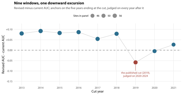
7 of the nine splits favour the revision, by 0.03 to 0.09; one is indistinguishable from a tie; and the published one is the only clear reversal — in Figure 15.1 it is the single point below the line, and not marginally. The panel thins as the cut year moves later — 9 / 47 sites at the start against 5 / 41 at the end — so none of these is a precise number, which is rather the point.
The revision’s discrimination advantage is not established, in either direction. It is positive on most forward splits and negative on the one reported above, whose own interval runs -0.16 to +0.02 (DeLong p = 0.22). A statistic that ranges -0.06 to +0.09 across nine reasonable windows on the same data and the same two indices is not measuring a difference between the indices. This is the same conclusion Section 13.5.5.1 reaches from the other end — criterion 1 cannot referee this contest — and the sweep supports it better than any single split does.
15.4.1.2 The other artefact channel: visits to a creek that is not flowing
Criterion 4 above is one channel — how many animals ended up in the tray. Chapter 13 turns up a second (Section 13.5.6.2): the published score is lower on visits where the creek was not flowing, by about a third of a standard deviation, which is a condition of the visit rather than a property of the creek. Freedom from artefact is the whole of the case for the revision, so a second artefact channel is worth checking before anyone acts on that case.
| Specification | Current system | Revised system |
|---|---|---|
| Site and year random effects | -0.32 (-0.551 to -0.095) | -0.06 (-0.302 to +0.183) |
| Site fixed effects | -0.30 (-0.530 to -0.069) | -0.05 (-0.291 to +0.199) |
| No year term | -0.35 (-0.585 to -0.112) | -0.20 (-0.456 to +0.051) |
| Month random effect added | -0.35 (-0.577 to -0.127) | -0.09 (-0.325 to +0.154) |
The incumbent’s step is there on all four specifications and the revision’s is on none of them. Freeing the six flow levels rather than fitting a line through them, the current score separates them (\(\chi^2\) = 14.01 on 5 df, p = 0.02) and the revised score does not (8.43, p = 0.13).
The revision does not carry the no-flow artefact the incumbent carries, and that is a point in its favour on criterion 4 — but do not lean hard on it. Fitted sample by sample on the same visits, the revision is +0.25 standard deviations less depressed at no flow than the current score, with an interval of +0.028 to +0.472 (p = 0.027) — the improvement itself only just excludes zero, on 39 no-flow samples at 34 distinct visits. That “only just” is doing real work and the model behind it matters: drop the visit random effect and the same contrast is +0.21 (-0.003 to +0.421), which covers zero. Flow state is a property of the visit, so the specification with the visit level is the right one and it is the one reported — but a positive demonstration that turns on one random effect is not a result to lean on. What can be said cleanly is the negative, and it holds under every specification in Table 15.13: nothing here suggests the revision inherits the channel, which is what would have undercut the case for it.
Where the difference comes from is worth a sentence, because the obvious explanation is wrong. Three of the four current factors fall at no flow (Section 13.5.6.2), and two of them are the raw family count and the raw EPT family count — the two the revision replaces with rarefied counts. The rarefied family count does not fall: +0.17 standard deviations (-0.15 to +0.50), and none of the revision’s four factors moves at all. But that is not because a dry creek gives up fewer animals — sample abundance is no lower on those visits (-0.03 log units, -0.22 to +0.15). So this is a second channel rather than the effort channel in disguise, and why rarefying closes it is not something this data can answer.
Neither system is reliable enough to support a five-class published rating from one sample. That is the finding of Section 13.5.1 and no change to the index repairs it. Neither reaches Test 2’s 20% class-change threshold on three samples either — the figures are 41% and 46%, both more than double it. That is this chapter’s own result and it is the reason two of the report’s suggestions do not wait on anything decided here: R1 and R1b in Section 19.4 state them, size what three samples buy, and carry these two figures as the evidence that the revision does not repair the problem. Section 13.7 works through the second of them — fewer published words, or a score with an uncertainty band instead of a word.
15.4.2 Which sites change, and by how much
| Current rating | Very Poor | Poor | Fair | Good | Excellent |
|---|---|---|---|---|---|
| Very Poor | 0 | 0 | 0 | 0 | 0 |
| Poor | 0 | 3 | 0 | 0 | 0 |
| Fair | 0 | 7 | 23 | 1 | 0 |
| Good | 0 | 0 | 7 | 20 | 0 |
| Excellent | 0 | 0 | 0 | 12 | 3 |
27 of 76 sites (36%) change class: 26 fall one class, 1 rise, and 0 move by two (Table 15.14). A further 1 site cannot be given a class under the revision, and the rarefaction threshold of Section 15.3.4 — whose samples, as that section shows, are not a random selection — accounts for 0 of it. The remaining 1 has a revised score that the published class table has no word for, because that table is not a partition: Fair closes at 2.99 and Good opens at 3.00, and the same 0.01-wide gap sits at 1, 2, 4 (Section 13.5.7). The published four-factor average is a multiple of an eighth and can never land in one; the revised score is continuous, and 12 of the 1,473 per-sample revised scores do. Those 4 gaps are now asserted where the table is defined, so they cannot be quietly closed — which would be re-scoring a published system — or quietly grow. The rank correlation between the two sets of site scores is 0.92 — the revision does not reshuffle the network, it recalibrates it. It does move individual creeks, though: 19 sites shift more than ten places in a network of 76, the largest shift is 21 places, and about one site pair in 8 reverses.
Almost all of the downward movement is the recalibration of Section 14.3 rather than the new factors: applying only the band reset, with the four original factors unchanged, already moves 27 of 77 sites (35%) down one class (Section 14.4.2).
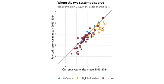
| Site | Waterway | Tier | Current | Revised | Imperv. % |
|---|---|---|---|---|---|
| 28.2EHZR | Ingar Creek | Reference | 2.96 (Fair) | 3.26 (Good) | 0.0 |
| 48NGK | Lapstone Creek | Urban | 2.00 (Fair) | 1.33 (Poor) | 26.5 |
| 45NBX | Cripple Creek | Urban | 2.04 (Fair) | 1.76 (Poor) | 7.8 |
| 57ELW | Cataract Creek | Urban | 2.11 (Fair) | 1.43 (Poor) | 20.8 |
| 58BLA | Leura Falls Creek | Urban | 2.15 (Fair) | 1.21 (Poor) | 32.0 |
| 86BKT | Kedumba Creek | Urban | 2.30 (Fair) | 1.96 (Poor) | 44.3 |
| 50NEP | Knapsack Creek | Urban | 2.33 (Fair) | 1.82 (Poor) | 18.2 |
| 26GWF | Water Nymphs Dell | Urban | 2.44 (Fair) | 1.64 (Poor) | 24.8 |
| 82EBB | Bedford tributary @ Albert Rd Bullaburra | Urban | 3.00 (Good) | 2.54 (Fair) | 7.1 |
| 59.2BLA | Leura Falls Trib u/s Chelmsford Dr | Urban | 3.04 (Good) | 2.70 (Fair) | 36.1 |
| 51NGK | Glenbrook Creek | Slightly disturbed | 3.07 (Good) | 2.79 (Fair) | 1.9 |
| 08GBH | Bridal Veil Creek | Urban | 3.33 (Good) | 2.74 (Fair) | 12.0 |
| 23.2BWF | Jamison Creek | Urban | 3.34 (Good) | 2.96 (Fair) | 18.6 |
| 74EBB | Bedford Creek Tributary @ Red Gum | Urban | 3.35 (Good) | 2.83 (Fair) | 16.2 |
| 18BKT | Megalong Creek tributary | Slightly disturbed | 3.50 (Good) | 2.82 (Fair) | 7.8 |
| 01CMW | Waterfall Creek | Slightly disturbed | 4.00 (Excellent) | 3.19 (Good) | 5.3 |
| 35GFB | Linden Creek tributary | Slightly disturbed | 4.04 (Excellent) | 3.96 (Good) | 8.2 |
| 31EHZ | Terrace Falls Creek | Slightly disturbed | 4.05 (Excellent) | 3.85 (Good) | 7.4 |
| 13BMG | Pulpit Hill Creek trib | Slightly disturbed | 4.08 (Excellent) | 3.46 (Good) | 5.0 |
| 34GWD | Woodford Creek | Slightly disturbed | 4.08 (Excellent) | 3.63 (Good) | 9.6 |
| 78GLN | Bulls Creek | Slightly disturbed | 4.11 (Excellent) | 3.60 (Good) | 6.8 |
| 03BMV | Fairy Dell Creek | Slightly disturbed | 4.26 (Excellent) | 3.37 (Good) | 11.7 |
| 11BMG | Megalong Creek | Urban | 4.33 (Excellent) | 3.53 (Good) | 1.2 |
| 10BMG | Pulpit Hill Creek | Slightly disturbed | 4.39 (Excellent) | 3.31 (Good) | 2.8 |
| 72NSP | Glenbrook Creek | Slightly disturbed | 4.39 (Excellent) | 3.58 (Good) | 1.8 |
| 80BMG | Back Creek | Slightly disturbed | 4.43 (Excellent) | 3.40 (Good) | 1.7 |
| 30EHZ | Bedford Creek | Slightly disturbed | 4.54 (Excellent) | 3.93 (Good) | 4.3 |
One site in Table 15.15 deserves comment, and one site that is not in it deserves more, because between them they are the kind of case you will be asked about.
28.2EHZR rises, and it is a reference site — the only site in the table that rises at all. The other case is 75BKTR (Reedy Creek), a reference site whose catchment burnt 100% in 2019–20 — and it is not in the table, because both systems already rate it Fair: 2.48 on the current score against 2.36 on the revised one, the same word either way. Adopting the revision does not put this reference creek below Good; the current system already does, and that is chapter 12’s tier finding rather than anything this chapter proposes.
The fire is not the explanation, and that is worth saying before it is offered as one. All 6 of the site’s samples in the 2015–2024 window were taken before the fire started on 4 January 2020, the last of them in October 2019, so the mean being rated contains no post-fire sample at all. Whatever puts this creek below Good is in its pre-fire record — and that is exactly the case where you must be able to say why the number is what it is, which is an argument for publishing the four factors alongside the composite rather than the composite alone.
15.4.3 Continuity
A revision that reclassifies 36% of the network overnight is politically hard, and it should be said plainly that this one does. Three things make it manageable.
- The ranking is largely preserved (rank correlation 0.92); the whole scale shifts down and stretches. It is not order-preserving, and the snapshot should not claim it is: about one site pair in 8 reverses, and 19 sites move more than ten places in a network of 76, the largest by 21 places. Individual creeks will move relative to one another; what does not change is the broad ordering of the network.
- The movement is almost entirely the band recalibration, which is correcting a documented error in the published urban bands, not a change of opinion about what health means.
- The direction is one-way and small. 26 sites fall one class, 0 fall two, 1 rise.
The transition itself is the fourth suggestion in Section 15.6, and it is the one piece of this chapter that is about communication rather than measurement: publish both ratings for one reporting cycle, label the old one as such, and say in the snapshot that the change is a recalibration of the scale rather than a decline in the creeks. The alternative — leaving the bands as they are because moving them looks bad — means continuing to publish a scale that is more generous than it says it is.
15.5 What we can and cannot say
| Question | Answer | Confidence |
|---|---|---|
| Does the revision remove the laboratory-effort artefact? | Yes, and this is the whole case for it. With site and year fixed effects the current score moves +0.41 (+0.34 to +0.47) standard deviations per natural-log unit of animals counted; the revision moves +0.03 (-0.04 to +0.10), an interval that covers zero. Across the interquartile range of sample abundance the current published score moves 0.41 points (0.36 to 0.46) with no change in the creek, and 0.60 points between creeks. | High. Two specifications, same direction, intervals reported. |
| Does it discriminate better? | Not established. Reference against urban goes 0.76 to 0.85, but on 11 reference sites the site bootstrap and the DeLong test disagree (p = 0.07), the good-condition comparison does not move, and the comparison is not stable to the evaluation window: on 2020-2024 site means the current system is ahead (0.78 against 0.72, interval -0.16 to +0.02), and on 7 of nine forward splits the revision is (Section 15.4.1.1). | Low, and it cannot be raised by re-analysis. Relabelling two sites in 63 moves the AUC by 0.08 (Section 13.5.5.1) — the same order as the contest. |
| Is it more reliable? | No, essentially unchanged. The intraclass correlation goes 0.49 to 0.44 and the single-sample class-change probability 60% to 65%. | High that it is not worse and not better. |
| Where is it worse? | On two criteria, both slightly — independence and boundary sensitivity. Independence: effective dimensionality 2.59 to 2.27. Boundary sensitivity: 9.4% to 10.7% of ratings change under a 0.1 shift, so the revision fails Test 6’s 10% mark and the incumbent passes. Responsiveness to catchment fire used to be counted here as a third and is not: neither response clears zero once it is fitted at the catchment and the year, where burn extent varies (Section 13.5.6), and a test of the DIFFERENCE gives +0.09 (-0.09 to +0.28), so the two are not distinguishable (Section 15.4.1). | High on the numbers, moderate on what they mean. The incumbent passes Test 6 because averaging eight integers quantises the score onto a 0.125 grid, which is not a virtue. Neither surviving criterion is a reason not to adopt the revision; both are reasons to publish the score beside the word. |
| What does it cost in coverage? | 30 of 1,503 samples (2.0%) hold fewer than 20 animals and cannot be rarefied, including 9 of the 31 Very Poor samples in the analysis set — 29% of the bad news this chapter can see, and that 31 is the narrowest of the report’s Very Poor counts (Section 15.3.4). Depth 15 halves the loss and buys nothing back; nothing makes it go away. | High. Counted directly, and the whole system was rebuilt at four depths to check that the choice is not doing the work. |
| Would it reshuffle the network? | No. 27 of 76 sites (36%) change class on 2015-2024 means, 26 down one, 0 down two, 1 up, and the rank correlation between the two sets of site scores is 0.92. Most of that movement is chapter 14’s band reset, not the new factors: the reset alone already moves 27 of 77 sites down. | High on the ranking, moderate on individual creeks — about one site pair in 8 reverses and 19 sites move more than ten places. |
| Is either system good enough to publish five words from one sample? | No, and no change to the index fixes it. The class-change probability on three samples is 41% for the current system and 46% for the revision, both more than double Test 2’s 20% mark. Reaching it on five classes would need about 13 samples (10 to 20 on a parametric bootstrap of the fit). | High. This is chapter 13’s variance decomposition (Table 13.6), read not refitted. |
| Should water quality, shading, rare families or network position go in? | No to water quality, shading and rare families, and no to a community change factor and to aggregating by minimum. Network position is deferred rather than refused: the expectation model it calls for needs catchments that are not delineated, but the interim step — splitting the anchors by distance from source, once there is a defensible place to cut — is recommended. Each is settled on its own evidence in Section 15.3.6, and three of the six have a better home outside the rating — a report card, a flag, and a habitat assessment. | Moderate to high, and each refusal carries its own interval. |
15.6 Four things you might want to think about
The numbering is that of Section 19.4, so these mean the same thing here as they do there. All four are suggestions. The evidence behind them is not soft, and none of the framing below is meant to make it sound softer — but which trade to take is a decision about what your rating is for, and that is not ours to make.
- Publish the rating from a rolling three-year window, not from one sample (R1). The cheapest of the four by a distance, and the only one here that does not turn on anything this chapter measures — which is why the whole of it is stated in Section 19.4 rather than restated here. R1 sizes what three samples buy, says what it costs, and says why the honest version is “much better” and not “solved”.
- Replace the two count factors with rarefied versions, and SIGNAL-SF with the tolerant share on SIGNAL 2 (R2). This is the part with a real trade in it. You buy freedom from an artefact that is documented, large and currently unmanaged; you pay 30 unrateable samples, most of them at the bad end, and you accept a change that has not been shown to discriminate better. You do not pay responsiveness for it. An earlier version of this chapter said you did, on a sample-level fit that did not survive being refitted where burn extent actually varies: neither response now clears zero, and the two are not distinguishable from each other (+0.09, -0.09 to +0.28; Section 15.4.1). That is one fewer stated cost, not a fifth argument for the change. Our view is that the artefact is the more serious problem, because it is systematically getting worse as the laboratory counts more animals — but it is a view, not a finding.
- Score each factor once between two anchors (R3), and if you do the band reset, do this with it (R4a). The two-anchor rule is worth having on its own — it gives the score a plain reading the percentile bands never had, and the gaps and overlaps in the published table cannot recur — and Section 15.3.3 sets out why chapter 14’s reset needs it alongside.
- Whatever you adopt, publish both ratings for one reporting cycle and label the change a recalibration. This is the one item here that is about communication rather than measurement, and it is the one most likely to decide whether the rest survives contact with a council meeting (Section 15.4.3). Publish the four factors and the score beside the word too:
75BKTRsitting at Fair — which it does under both systems, not because of anything proposed here (Section 15.4.2) — is defensible the moment you can point at the four numbers behind it, and indefensible if all anyone can see is the word. It is not defensible by pointing at the fire: that catchment burnt after the last sample in the window the rating is computed over (Section 15.4.2), which is precisely why the factors have to be publishable and not just the composite.
And one thing that is not a suggestion, because it is a question rather than an answer: five words may be more than the data can carry. Section 13.7 works through what fewer classes, or a score with an uncertainty band instead of a word, would buy. Nothing in this chapter depends on the answer, and both systems have the same problem.