Blue Mountains Healthy Waterways

Statistical analysis of macroinvertebrate and water quality monitoring, 1998–2025

Preface

Blue Mountains City Council has been sampling the animals that live in its creeks, and testing the water they live in, since 1998. This report is the first full statistical analysis of that record.

It covers 2,062 macroinvertebrate (“waterbug”) samples taken at 134 sites between October 1998 and August 2024, and 2,688 water quality samples taken at 135 sites between January 1998 and June 2025. Both were supplied as Microsoft Access databases in July 2025 and are reproduced here without alteration. To these we have added catchment information that Council’s databases do not hold — imperviousness, rainfall, drought and fire history — built from public Australian government data.

You asked a set of questions — whether the creeks are getting better or worse, whether water quality is changing, what drives the differences between creeks, and whether the waterway health rating you publish each year is doing its job. This report answers them, and it does one thing you did not ask for. Nobody had audited these two databases end to end, and a good deal of what follows is a report on the monitoring program itself: what it measures reliably, what it does not, and what would need to change.

This is written for you — the Healthy Waterways team. It assumes you know the creeks and the bugs, so it gives you no background there. It does not assume you spend your days doing statistics, so where a result turns on a statistical argument the argument is spelled out rather than asserted. The summary that follows keeps to the numbers that carry the story; the chapters have the rest.

Every number, figure and table in the report is generated from the source data by code held in the project repository, and rebuilding the report rebuilds them. The executive summary works the same way, and every figure in it is now either computed here or read from the very fit the chapter used, so the summary and the chapter cannot drift apart. Rebuilding instructions are in README.md.

How the report is arranged

Nineteen chapters in four parts, and one appendix (Table 1).

Table 1: How the report is arranged.

	Chapter	What it covers
I	1. The monitoring record	What the two databases hold, how they link, what had to be repaired, and the proof that Council’s published calculations reproduce exactly.
	2. What we need from you	The master list: everything the analysis had to guess at, ranked by what it would buy against what it would cost you.
	3. How the method changed	Every documented and undocumented change to how the creeks were sampled and measured, and what each one costs the record.
	4. Catchments, climate and fire	Imperviousness for every site, rainfall and drought, and fire history — none of it in Council’s databases, all of it built from public data.
II	5. Has waterway health changed?	Has the published health score moved? Over what period? Is the change real?
	6. Water quality: what changed	Have the eleven measured parameters changed, overall and site by site?
	7. The water quality report card	How often readings sit inside your own desirable ranges, and what a published report card could honestly say.
	8. What lives in the creeks	Which animals are there, how that has changed, and which families are winning and losing.
	9. Why the creeks differ	What explains the differences between creeks — habitat, water quality, catchment, and who filled in the field sheet.
	10. The rare families	The animals a condition rating cannot see, the creeks that hold them, and what to do about it.
	11. The wetlands	Nine sites that are not streams — a lagoon, a lake, a dam and one swampy creek reach — scored as though they were one kind of thing.
III	12. An external check	An independent scheme’s verdict on the reference sites the whole rating is calibrated against.
	13. Is the current rating any good?	Reproducibility, what the four factors actually measure, and how well the rating separates a reference creek from an urban one.
	14. Resetting the percentile bands	What a reset would do, and whether the 2019–20 fires make it unsafe.
	15. A revised rating	A four-factor revision, and an honest comparison against the current system.
	16. How to test any future rating	Six tests, as a protocol you can run against any draft, including this one.
IV	17. Evaluating the works	Why the stormwater treatment projects cannot be evaluated from the record, and what a design that could would cost.
	18. What to measure next	The monitoring questions worth answering, and the smallest change to the program that would answer each.
	19. Conclusions	The findings drawn together, and the recommendations with their reasoning and cost.
A	The data layer	How the databases were read, repaired and joined; the standing limitations; the technical reference.

Chapters carry limitations where they belong, and Appendix A holds the 16 that apply to the whole report. They are not buried; they are the most useful part of the document for anyone planning the next ten years of monitoring. Chapter 2 is the one to send to your team: it collects the 130 things this analysis had to guess at, work around or leave open, each written as a question somebody at Council can answer.

Executive summary

The short version

Blue Mountains creeks are in better shape than they were at the start of the record, and nothing detectable has happened to them for about the last decade. The improvement was real, it was not simply the drought breaking, and it shows up in the animals rather than in the water chemistry.

One thing had to be taken out of the record before that sentence could be written. Until 2007 the field team also sampled riffles — the fast, stony water — and after 2007 it stopped. A riffle sample scores about a quarter of a rating point above the edge sample taken beside it on the same day, so the habitat that was dropped is confounded with the very question of whether health has changed since the 1990s. It works against the finding rather than manufacturing it, but a confound that happens to point the helpful way is still a confound. Everything below is measured on the edge samples alone, which is the one consistent series the archive contains.

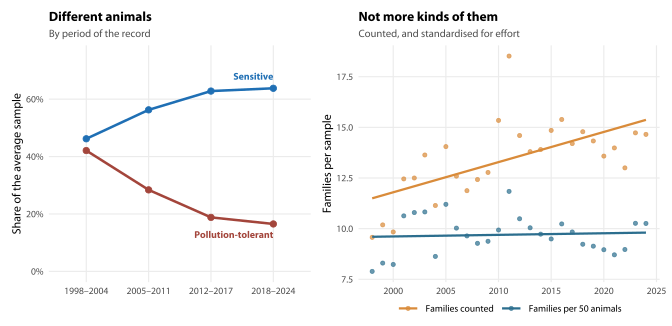
But the improvement is not the one the numbers appear to describe. The creeks are not carrying more kinds of animal than they used to — and over the last decade they have been carrying fewer. They are carrying different animals: the tolerant species that survive in poor water have been replaced by sensitive ones that cannot. Over the record the average sample’s share of animals belonging to pollution-tolerant families fell from 42% to 17%, while the share belonging to sensitive families rose from 46% to 64%. That is the single clearest signal in twenty-six years of macroinvertebrate sampling, and it is the result that moved least under testing: standardising for how many animals the laboratory happened to count costs it 5.8% of its size and nothing else. The health rating does not report it.

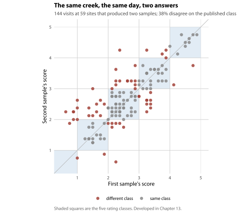
The rating system needs work, and the most valuable fixes are cheap. Two samples taken from the same creek on the same day give a different published rating nearly four times in ten — 38% of 144 such visits at 59 sites (95% confidence interval 29% to 47%), and 59% of the 39 visits rated Poor. Publishing the rating from three years of samples instead of one is a large improvement and not a cure: it cuts the modelled probability that a re-measurement changes the published class from 60% to 41%, and it costs nothing but a change to a database query. The other half of the fix is to publish fewer words: five classes are more than these creeks can be sorted into reliably.

And there is something the rating is not looking for that the creeks are measurably losing. The rare families — the ones found in fewer than twenty samples in the whole archive — are disappearing, at about a fifth per decade, and the loss is steeper still when every sample is standardised to the same number of animals. The condition rating cannot see them, because several of the creeks that hold them do not rate as being in good condition. Chapter 10 names the ten creeks concerned and argues for a protection tier separate from the condition rating; Chapter 19 carries it as a recommendation. This is the recommendation most likely to change what you actually do, and it was not one you asked for.

The four claims, in three pictures

The rest of this summary is the argument. These three figures are the evidence for it, and between them they carry the whole story.

Figure 1: Waterway health improved for the first half of the record and then stopped. Each point is the average across sites of that year’s mean health score; the line is a two-piece fit that estimates where the improvement ends rather than assuming a date, and the dashed line is that estimate. The shaded band around it is the uncertainty in the date, profiled from a second fit which carries the year effect the two-piece fit cannot — so the band and the dashed line come from different fits, 0.1 of a year apart and in the same calendar year. After it, nothing can be detected in either direction — which is not the same as nothing happening.

Figure 2: The improvement is a change of cast, not a change of headcount. The share of each sample made up of pollution-tolerant families has more than halved, and the sensitive share has risen to match; but standardise every sample to the same number of animals and the number of families found shows no net change in twenty-six years of sampling — and falls 0.85 families per decade over 2010–2024 (0.05 to 1.65) — a fall that is in the scatter of the right-hand panel rather than in the straight line drawn through it.

Figure 3: Why the published rating needs more than one sample. Each point is one visit on which the field team took two samples from the same creek on the same day, with one sample’s score against the other’s. Points off the shaded diagonal are visits where the two samples fell in different published classes — nearly four in ten. The bands are narrower than the difference between two samples of the same creek.

Your questions, answered

You asked ten questions. Two of them turned out to be one question asked twice, and one — whether the climate data exists — was answered by building it, so its interesting half is asked here instead. That leaves nine.

1. Has waterway health changed over time?

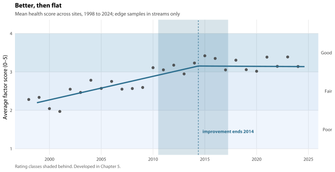
Yes, and the improvement stops about 2014. Averaged across the whole record the health score improves by about two fifths of a rating class per decade (0.40 score points per decade on the 0 to 5 scale, 95% confidence interval 0.30 to 0.51, where one rating class — Fair to Good, say — is 1.00 score points wide). Rather than splitting the record at a round number, the analysis estimates where the improvement ends, and puts it at 2014.4. Where it lands is solid — drop any single year of the record and the answer moves by less than half a year. How tightly it can be bracketed is a different question, and a looser one: once a whole field round is allowed to share its weather and its crew rather than counting as thirty to ninety independent observations, the 95% interval runs from 2010.5 to 2017.25. That interval is a likelihood profile, a separate fit from the one the estimate comes from, because the estimator itself cannot carry a year effect; the profile puts the change at 2014.5, 0.1 of a year away and in the same calendar year, and 2014 is what the record is split at. Before that point the score climbs steeply; after it, nothing can be detected either way. This is not the drought breaking: adding rainfall and drought indices to the model changes the answer by nothing of consequence. Figure 1 is the picture.

One caution about the flat decade. “No change detected” is not the same as “no change”. The record since the changepoint is short enough that a decline of up to 0.46 score points per decade would still have gone unnoticed — and an improvement of up to 0.22, which is the after-the-changepoint row of Table 5.3. The two bounds are not the same size, and the larger one is the one that should worry you. Developed in Chapter 5.

2. Have the four parts of the health score changed — and is the fall in family counts bad news?

Yes to the first, and no to the second. The four factors have not moved together, which the single averaged score conceals entirely. Over the whole record the rise in the number of families found per sample is mostly a counting artefact; the rise in mayflies, stoneflies and caddisflies is mostly real; and of the two sensitivity indices, the one Council’s rating uses moves only about a quarter as far as the standard one does on the same animals. Since the changepoint the family count has clearly fallen while Council’s sensitivity index has drifted up. Averaging four measurements of that kind gives each equal weight regardless of what it is measuring, and the composite reads flat.

The falling family count is the clearest good news in the report, not a warning. Of the families lost per sample since 2010, 60% are families graded as pollution-tolerant. That share is known to within about 40% to 106%, from resampling whole creeks — which is the sampling uncertainty, and it is wide. A limit above 100% is not an arithmetic slip: in 3.3 per cent of resamples the intermediate and sensitive families gained ground while the tolerant ones fell, which puts the tolerant loss above the net total. Two further choices move it again — the share runs 37% to 81% as the tolerance boundary is swept a grade either way, and the loss it is a share of depends just as much on starting the clock at 2010. What none of them move is the direction: the total fell in every one of the 600 resamples, and sensitive families have not declined at all under any of those choices. The creeks are shedding the animals that indicate poor water — which is the right-hand panel of Figure 2 seen from the other side. One qualification belongs with it: that decomposition is of the recorded family count. The effort-standardised count falls over the same decade too, and nobody has yet tested whether that fall is also confined to the tolerant families. So “good news” is the reading the evidence points to, not a result in its own right. Developed in Chapters 5 and 8.

3. Has water quality changed over time, and at which sites?

Mostly it has not changed in any way that can be separated from changes in how the measurements were taken. Of the eleven parameters of Table 6.6, exactly one shows a trend that survives every check: water temperature is rising by about half a degree per decade (0.31 to 0.85 °C) averaged over the year — the warmer half is warming about three times as fast as the cooler, at about a degree per decade against about a quarter, so the single rate is an average over a sampling calendar rather than a rate the streams have anywhere in particular (The trend summary). Even that deserves a footnote, because the gridded air temperature record for the same catchments over the same years does not confirm it. The large apparent improvements in dissolved oxygen and turbidity are step changes at the 2017 and 2020 probe replacements, not changes in the creeks, and once the steps are allowed for no residual improvement can be established. Conductivity, alkalinity and nitrate show no detectable trend, which is not the same as no trend: conductivity in particular is estimated at a 14% rise per decade with a range running from a 3% fall to a 34% rise, wide enough to be consistent with a genuine salinity problem.

There is one robust piece of good news. Measurements are more often inside your own desirable ranges than they used to be: 65% over 2022 to 2025 against 54% over 2002 to 2005, across 11,178 measurements at 122 sites, and the improvement is indistinguishable in urban catchments and reference ones. Two of the parameters carrying it are the two whose measurement changed most, so that caveat should travel with the figure — but the improvement survives removing them.

At individual sites, nothing can be established. 648 site-by-parameter tests were run and not one survives once the chance of a false positive across that many tests is controlled for, and no creek should be singled out for inspection on that basis. Site-level water quality reporting is worth resuming once the sampling calendar is fixed, the instrument is stable or overlapped at each change, and a set of sites carries a guaranteed water quality sampling frequency — but not before. That last one is not the core_reporting designation you already hold: that is a macroinvertebrate reporting subset and it carries no schedule, so the requirement is a different list and a different commitment. Developed in Chapters 6 and 7.

4. Are there correlations with imperviousness, and can we get a more accurate figure for every monitoring site?

Yes to both, with one important qualification about how the figure should be used. Imperviousness — the share of the catchment under roofs, roads and pavement — is the strongest catchment-scale predictor in the report. Waterway health falls by about 0.035 points of score for every additional percentage point of the catchment sealed, and nothing in this record marks a level at which the harm switches on: Table 5.13 carries the same loss per percentage point in every band of the gradient. The honest statement beside that rate is chapter 5’s: the decline is clear across the network as a whole and not detectable below about 10% sealing, where the same regression on the 54 sites below that line returns -0.013 per percentage point (-0.084 to 0.057, p = 0.71). 54 of the 117 sites sit below 10% sealed, so over that half of the network this record can neither show the decline separately nor refute it — a constant decline is not established down there, and it is not ruled out either. The analysis supports ranking catchments by imperviousness; it does not support any numeric planning trigger, and “harm accrues from the first few per cent” rests on the whole-network slope and on King et al. (2011) rather than on a measurement of that stretch.

Where the low end has been tested directly, on far more streams than we monitor, the literature is blunter than that and points the same way. King et al. (2011) looked at 1,939 Maryland stream reaches and found the declines were not scattered along the gradient at all: 110 of 238 animal groups fell away together, at community-level thresholds of 0.68%, 0.96% and 1.28% impervious cover in the three regions they cover, with the upper confidence limit below 2% everywhere. A threshold at about one per cent of the catchment sealed is not a planning trigger. It is far below any level a planning instrument could sensibly use, and well below what a network of this size could resolve — so the practical conclusion is the same one: rank the catchments, and do not wait for a number to be crossed.

Neither Council database holds an imperviousness figure, so one was built: the upstream catchment of every suitable site was delineated from the national elevation model, and imperviousness estimated from land use, road corridors and address density. It covers 126 of the 134 macroinvertebrate sites — Table A.2 says which population each of those counts is out of. The eight register sites it misses are not missing coordinates — every site has an easting and a northing — they are sites whose catchment could not be delineated reliably, so they are withheld rather than guessed at.

Treat the check on that figure as a consistency check rather than a validation: all fifteen reference sites whose catchment could be delineated come out at effectively zero, but fourteen of the fifteen contain no address points at all and the one that does holds three over 1,870 hectares, and address points are one of the inputs, so the test could not have failed. The ranking is usable. The absolute values are not. Turning a modelled figure into a measured one needs two datasets you already own — the stormwater pipe and pit network, and a record of which streets are kerbed (dq:complete-drainage-network, dq:measured-road-surface-areas). Developed in Chapter 4.

5. What did the 2019–20 fires do to the benchmark the ratings are judged against?

This was not one of the ten questions. It should have been.

Nine of the fifteen reference catchments that could be delineated had more than 90% of their area burnt in the 2019–20 Black Summer fires, and five reference catchments burnt over more than half their area twice in seven years; Table 4.17 is the catchment-by-season record both counts are taken from. The reference sites are the benchmark against which every Excellent rating is judged, and that benchmark has been through two fires since it was set. It moved: where the catchment burnt, the rating fell by 0.47 points relative to the unburnt reference creeks over the same years (95% CI 0.04 to 0.90) — about half a rating point, on an interval wide enough that “about” is doing real work.

How much it moved depends on how burn extent is measured. Taking it from each sample’s own three-year fire history rather than from the 2019–20 season alone gives a smaller loss, on an interval that reaches past zero. The direction does not change, and where the two periods are cut is not a free choice at all — every 2020 sample at a burnt site was taken after the fires had started. The half-point figure belongs to the 2019–20 measure and should be quoted with it.

The climate half of the original question is simply answered: daily rainfall, temperature and drought indices for every site and every sampling date have been built from the national SILO surfaces, and fire history for every catchment from the NSW fire history layer. They exist, they are in the repository, and they are available to any future analysis. Developed in Chapters 4 and 14.

6. Have the stormwater treatment projects achieved change?

This cannot be answered, and no amount of analysis will change that. Evaluating a treatment device needs four things: samples before the works, samples after, matched untreated control sites, and a date. The databases hold no commissioning dates, no control sites were designated, and the Kedumba monitoring sites were established in 2022, after the works. Fabricating an intervention date and fitting a model to it would produce a number that means nothing.

What can be said is that the treated catchments are exactly where Council’s own framework says works are warranted, and that a future evaluation is possible if it is designed rather than assembled afterwards. It is not cheap. Detecting a change of half a score point needs about twelve treated and twelve control sites, each sampled twice a year for six years either side of the works — not four sites per arm, at which half a score point cannot be detected at any amount of sampling, because creeks differ too much in how they change (Table 17.6). The best the existing record manages is 0.65 score points on 3 treated sites against 9 controls, which is larger than any effect worth finding.

If twelve sites in each arm cannot be resourced, Chapter 17 sets out three alternatives — measure something that varies less between sites, pool several works programs into one evaluation, or accept in advance that the evidence will be descriptive. What is worth avoiding is a four-site study whose null result gets reported as “no effect”. The commissioning dates are the first thing to fix for this question — nothing else about the works evaluation can be settled before them (dq:sqid-commissioning-dates, dq:stormwater-eval-design-decision). They are not the report’s first thing to fix; Where to start below is that list. Developed in Chapter 17.

7. Which water quality and physical site characteristics most influence the animal communities?

Physical habitat — ahead of water quality, ahead of imperviousness, ahead of the passage of time. Read that as an ordering and not as a set of sizes. Chapter 9 now tests the ordering against a null instead of assuming it, and the ordering holds; the sizes do not. More than half of what the physical habitat and water quality blocks each appear to explain on their own is what columns of pure noise of the same width earn, and that noise floor rises with the number of variables in a block, so two blocks of different width cannot be compared on that number at all. Of the things you can act on, catchment imperviousness ranks first and riparian shading second. Fine sediment on the creek bed ranks third and matters most for the rare animals.

The habitat data came from a source no analysis had previously used: the shading, substrate and vegetation observations your field officers have been writing on the water quality field sheet since 2006. Adding them, together with water quality, raises the amount of compositional variation the analysis can explain from 19% to 31%, and means that measured site variables now account for about three-quarters of everything that separates one creek from another. Both percentages are an upper bound: about a quarter of the dissimilarity the ordination works on is negative eigenvalue, which flatters any variance share read off it. On the conservative measure that removes it, the rise is 10.6% to 18.3% (Table 9.7 sets the two pairs side by side). The ordering — habitat first, then water quality, then imperviousness — is the same either way, and the ordering is what the recommendations rest on.

Within a single creek, almost nothing you measure predicts the difference between one visit and the next. The standing objection to that was always that the one thing worth measuring — how much water was in the creek — was not being measured. It was: a free-text box on the site description sheet has recorded flow state since 2008, and once tidied into a usable scale it accounts for 1.7% of the within-creek variation where it is recorded, 1.0% on its own, and 0.2% that nothing else already explains. The driver most often nominated as the missing one has been found, and it is the smallest thing on the list.

What does show up is who filled in the field sheet: for three of the 13 habitat variables the recording officer accounts for at least as much of the variation as the site does. That is an argument for the written protocol and photo points Chapter 18 recommends (dq:habitat-protocol-photopoints), not against using the data. Developed in Chapter 9.

8. What is special about the sites that support the rarer families?

It depends which rare families. For the sensitive ones, three site characteristics survive a proper test: a coarse, unsilted creek bed, catchment area, and dissolved oxygen. Fine sediment is the strongest of the three. The rest of the rare families are lowland still-water animals that are rare in the Blue Mountains simply because these creeks are steep and cold. Averaging the two groups together destroys the signal, which is why no previous summary has found anything.

Ten creeks carry most of the sensitive rare families (Table 10.7), headed by Pierces Pass Creek, Pulpit Hill Creek and Glenbrook Creek. Eight of the ten are urban or slightly disturbed creeks rather than reference sites, which is precisely why they matter: those are the places where protection has something to lose. The list stops at ten for a reason — below them, 29 of the 95 sites with enough samples to judge hold exactly one sensitive rare family each and cannot be ranked against one another, so any longer list is reporting a tiebreak as a rank.

One creek — Waterfall Creek — holds an established population of a freshwater amphipod family that includes short-range endemics elsewhere in the Sydney Basin: five records and 172 animals over 14 years. Knapsack Creek and Blue Gum Swamp Creek have each produced a single detection of three animals, once (Table 10.8). Those are worth looking for again; they are not second populations. Developed in Chapter 10.

9. How could the waterway health rating system be improved? Should water quality be part of it? Should the percentile bands be reset? Should a riparian and geomorphic rapid assessment follow? And what tests should we apply to a new draft?

The rating system is a reasonable design that has given Council a consistent language for a decade, and nothing in this report says it should be abandoned. It has three fixable problems: it is not reproducible on repeat sampling, two of its four factors partly measure laboratory effort rather than creek condition, and its sensitivity index sees only about a quarter of the change that has actually happened in these creeks. Each part of the question has its own chapter.

• Improvements (Chapters 13 and 15). Publish the rating from a rolling three-year window rather than a single sample; publish three classes rather than five, or publish the score and its uncertainty beside the word; replace the two count-based factors with effort-standardised versions; replace SIGNAL-SF with a measure built on SIGNAL 2; and always report the four factors alongside the composite. The case for changing the factors is that it takes the laboratory out of the score: sensitivity to how many animals were counted goes from +0.48 to +0.13 standard deviations of score per natural-log unit of animals, and — once the sampling year is allowed for, the cleaner comparison — from +0.41 to +0.03, which is no longer distinguishable from nothing at all. It does not lift the system’s ability to tell a reference creek from an urban one, and that should not be part of the case: the revision looks better (0.85 against the current system’s 0.76, the first row of Table 15.10), but it rests on the eleven reference sites carrying a rated sample in the evaluation window, against 52 urban ones — reference names several different site sets in this report, and Which sites are “reference”, and how many says which is which. The interval on the difference (+0.01 to +0.19) only just clears zero, and a DeLong test on the same pair does not (p = 0.07). Restricting the comparison to 2020–2024 site means reverses it (the revision 0.72 against 0.78) — on an interval of -0.16 to +0.02 that covers zero (DeLong p = 0.22), and it is one evaluation window of nine, seven of the other eight favouring the revision. One cost should be stated: the effort-standardised factors cannot rate a sample holding fewer than 20 animals, so 30 samples would go unrated, and nine of those are currently rated Very Poor. A suppressed rating must be published as suppressed, not quietly omitted.

• Water quality: no, not as a rating factor (Chapter 7). Publish it beside the rating as a separate report card scored against Council’s own trigger values — and score only alkalinity, nitrate-N and conductivity, with conductivity scored only within an instrument era, or against a baseline re-set at each changeover: it is the only one of the three read off the probe, and its level steps at both probe replacements (Chapter 6). Water quality is valuable because it says what is wrong; it does not separate creeks better than the animals already do, and 45% of macroinvertebrate samples have no same-day nitrate-N reading. Phosphate must not be published as a pass rate. 53% of the 1,127 phosphate readings in the archive are exactly zero — the test kit not detecting anything — and the desirable range starts at zero, so every non-detection counts as a pass. Report how often phosphate was detectable, say plainly that this is a property of the test, and do not score it. One thing about the parameter itself, because it is not in its name and it is not recorded anywhere: neither database says whether phosphate is reported as PO₄ or as P, and the two differ by a factor of three, so every phosphate figure in this report — here and in the chapters — is species-ambiguous (Phosphate: an exceedance rate that is really a detection rate). Nitrate-N declares its species; phosphate does not.

• Resetting the bands: yes (Chapter 14), on a rolling ten-year window of reference and slightly disturbed sites, as Council proposed, refreshed every five years. The reset would move 27 of 77 sites down one class — a correction to a scale that is currently more generous than it claims to be, not a decline in the creeks. An obvious worry is the fires, and it is a real one: the 2019–20 fires did lower the reference benchmark. They are still not a reason to delay. On a ten-year window, keeping the burnt catchments in the calibration set changes only 2.7% of rated samples and one site in 77, because the wet years that followed lifted the unburnt reference creeks by more than the fire depressed the burnt ones. Two conditions attach. The window must stay at ten years, and the band set that excludes the burnt catchments must be published alongside every reset, so that you can see what the fires cost.

• Rapid habitat assessment: yes, as a third panel, not as a rating factor (Chapter 18). You already collect most of one on the existing field sheet. What is missing is a written protocol, photo points, and consistent completion.

• Tests for a new draft: six of them (Chapter 16), as a standalone protocol you can run against any future version, demonstrated in the chapter by applying them to both the current system and the revision. The demonstration is not a formality: both systems fail the reliability test against its own standard, and the proposed revision fails the band-behaviour test where the current system passes.

Four things that were not on the list

These did not come from the questions. They emerged from the analysis, and each one changes how an existing number should be read. Each is also an entry on the master list in Chapter 2, because each of them is something only you can settle.

1. The laboratory is processing about twice as many animals per sample as it used to, and that alone raises the health score. The typical sample held 92 animals over 1998 to 2009 and 167 from 2014, with the rise concentrated in 2008 to 2011 — the same window in which the health score rose fastest. Two of the four scoring factors are counts of families, and the more animals you count the more families you find. About a third of the apparent improvement in the health score disappears once abundance is held fixed, and the whole of the apparent gain in family richness does: standardised to a fixed number of animals, family richness shows no net change in twenty-six years of sampling (0.05 families per decade, -0.39 to 0.50). That null is the average of a rise and a fall rather than the absence of both — over 2010–2024 the same measure falls -0.85 (-1.65 to -0.05), on an interval that excludes zero, and the raw count falls with it. That is the right-hand panel of Figure 2.

Neither database records a subsampling protocol or a target pick count, so we cannot say whether the creeks genuinely hold more animals or the laboratory is simply picking more of each sample. This is the largest unresolved confound in the report, and one field-protocol document from Council would settle it (dq:pick-count-protocol). (Chapters 3, 5 and 8.)

2. Two laboratory methods changed without being documented anywhere. Faecal coliform counts fall about a hundredfold across the summer of 2004–05 — at every site by the same factor, including reference sites in undeveloped bushland with no sewerage and no stormwater. A hundredfold improvement in untouched bushland is not an environmental result. Nor is it a decimal point in the wrong place: the numbers on both sides of the break sit on the same reporting grid, which a units slip could not do. Something changed about what was being counted. Separately, phosphate and nitrate results over 2017 to 2019 are not comparable with the rest of the series: phosphate jumps more than sixfold and returns almost exactly to where it started, and the share of results below the detection limit collapses and then recovers. That has the shape of a change of test kit or reagent.

Both were found in the data, not in any record. Council’s own purchasing and laboratory records would confirm them (dq:coliform-2004-break, dq:nutrient-2017-2019-change), and until they do, more than twenty years of coliform data cannot be joined into a single series. (Chapter 3.)

3. The published rating is not reproducible on a repeat sample. You have, without setting out to, collected the evidence: 144 visits at 59 sites produced exactly two samples from the same creek on the same day. In 38% of those visits the two samples fall in different published rating classes (95% confidence interval 29% to 47%). The figure is worst where it matters most: 59% of the 39 visits rated Poor, against 18% of the 11 rated Excellent. The rating classes are narrower than the natural variation between samples — Figure 3 shows exactly that. This is not a criticism of the field team; it is arithmetic, and it is the cheapest thing in this report to fix. (Chapter 13.)

4. SIGNAL-SF sees about a quarter of what a standard sensitivity index sees, and nothing that the standard index does not. The sensitivity index the rating uses has no grade at all for a good many of the recorded taxon names, and its grades are compressed at the tolerant end. Set the two indices side by side across every family whose fortunes were tested, and SIGNAL 2 accounts for about four times as much of which families are winning and losing as SIGNAL-SF does. Put both in the same model and SIGNAL-SF adds nothing at all. It scores mosquito larvae and diving beetles as though they were clean-water animals, so their disappearance barely moves Council’s index. The tolerant-to-sensitive shift is the largest signal in the dataset, and the rating’s sensitivity factor is a noisy version of a scale that would report it properly. (Chapters 8, 13 and 15.)

What this analysis cannot tell you

Nine things are worth stating plainly, because a reader who does not know them could take more from this report than it will bear. The first, second, fifth and ninth are gaps you can close; they are on the master list.

1. Whether the treatment works have worked. No commissioning dates, no control sites. This is a gap in the record, not in the analysis (dq:sqid-commissioning-dates).
2. Whether the doubling in animals per sample is real or procedural. No protocol was recorded. Everything that depends on counting is reported both ways (dq:pick-count-protocol).
3. Whether anything here is a cause. These are associations across creeks and across time. Creeks with high imperviousness differ from creeks with low imperviousness in many ways besides imperviousness, and no intervention appears anywhere in the record.
4. What is happening at any individual site’s water quality. The record will not support it, and this report names no site on that basis.
5. What phosphate is doing. 53% of the 1,127 phosphate readings in the archive are recorded as exactly zero, which almost certainly means the test kit did not detect anything rather than that there was nothing there. Until the detection limits and the kit history are confirmed, the phosphate series is as much a statement about the test as about the creek (dq:lab-detection-limits).
6. How much of the flat decade since 2014 is real. The record is long enough to say that no change has been detected and short enough that a decline of up to 0.46 score points per decade — or an improvement of up to 0.22 — could have gone unnoticed.
7. How fast the sensitive rare families are declining. The decline in rare families as a whole is solid and holds however the line between rare and common is drawn. The steeper figure for the sensitive ones does not: it depends on that line, and it reverses if the line is moved.
8. How badly the 2019–20 fires hurt the creeks, and how long recovery takes. One thing is now established — the fires depressed the reference benchmark where the catchment burnt. Whether the rating responds to catchment fire is not. Burn extent is a property of the catchment and the year rather than of the sample, and refitted at that level — 14 burnt creeks out of 83 — the estimate is -0.16 points with a 95% interval of -0.35 to 0.02, which covers zero (Responsiveness). What is not known is severity or trajectory: there are few post-fire samples, and the very wet years that followed are entangled with any recovery.
9. What lives in the creeks below family level. Everything here is family-level identification, which is the level your protocol records. The amphipod population in Chapter 10 needs a specialist to identify (dq:paramelitidae-verification).

Where to start

If you act on only three things from this report:

1. Record the pick count and the subsampling protocol on every laboratory sheet. This retires the largest single confound in the whole analysis (dq:pick-count-protocol, and dq:pick-count-field for the change to the sheet itself). Nothing on the master list buys as much for as little: this and item 2 below are two of the 3 asks tied at the top of Chapter 2’s ranking, each rated transformative and costing you minutes — the order between them is alphabetical by id, not a ranking.
2. Run the old and new instruments side by side for two field days at the next probe change. Two days of field time would convert most of Chapter 6’s “cannot be separated from the instrument” verdicts into correction factors, for this change and every future one (dq:side-by-side-runs).
3. Publish the rating from three years of samples, not one — and decide how many words the result should be reported in. A change to a reporting query, and the single largest improvement available to the reliability of the published rating. It does not finish the job: even on three years of samples, 41% of repeats would still change class — against 60% on the current one-sample practice, and against a standard of one in five. Getting to one in five on the current five-class scale would take about thirteen samples per rating — 10 to 20 once the uncertainty in that estimate is carried — which is not going to happen. On three classes it takes five. That is a decision about how you talk about your creeks, not a statistical one — but the statistics constrain it, and five words on one sample is not one of the available options.

Chapter 19 sets out the full set of recommendations, with the reasoning, cost and consequence of each. Chapter 2 is the list of things we need from you.

King, Ryan S., Matthew E. Baker, Paul F. Kazyak, and Donald E. Weller. 2011. “How Novel Is Too Novel? Stream Community Thresholds at Exceptionally Low Levels of Catchment Urbanization.” Ecological Applications 21 (5): 1659–78. https://doi.org/10.1890/10-1357.1.